Robot Applications
Copyright © 2014 Dr. Korondi Péter, Halas János, Dr. Samu Krisztián, Bojtos Attila, Dr. Tamás Péter

A tananyag a TÁMOP-4.1.2.A/1-11/1-2011-0042 azonosító számú „ Mechatronikai mérnök MSc tananyagfejlesztés ” projekt keretében készült. A tananyagfejlesztés az Európai Unió támogatásával és az Európai Szociális Alap társfinanszírozásával valósult meg.

Reviewed by: Dr. Husi Géza
Published by: BME MOGI
Editor by: BME MOGI
ISBN 978-963-313-136-7
2014
- 1. Introduction: Trends in robotics
- 2. Robot middleware
- 3. Universal robot controller
- 4. Internet-based Telemanipulation
- 4.1. Abstract
- 4.2. Introduction
- 4.3. General approach of telemanipulation
- 4.4. Master devices as haptic interfaces
- 4.5. Animation of the operator’s hand wearing the sensor glove
- 4.6. Overview of control modes
- 4.6.1. Basic Architectures
- 4.6.2. Nonlinear scaling (Virtual coupling impedance)
- 4.6.3. Time delay compensation of internet based telemanipulation
- 4.6.4. Friction compensation for master devices
- 4.7. A complete application example: A handshake via Internet
- 4.8. Conclusions for telemanipulation
- 4.9. References for telemanipulation
- 5. Holonomic based robot for behavioral research
- 6. Fuzzy automaton for describing ethological functions
- 8. Models of Friction
- 9. PCI universal motion control system
- 10. PCI CARD – Specifications
- 10.1. Pin-outs and electrical characteristics
- 10.2. Mechanical dimensions
- 10.3. Connecting servo modules
- 10.4. Axis interface modules
- 10.4.1. Typical servo configurations
- 10.4.1.1. Analogue system with encoder feedback
- 10.4.1.2. Incremental digital system with encoder feedback and differential output
- 10.4.1.3. Incremental digital system with encoder feedback and TTL output
- 10.4.1.4. Incremental digital system with differential output
- 10.4.1.5. Incremental digital system with TTL output
- 10.4.1.6. Absolute digital (CAN based) system
- 10.4.1.7. Absolute digital (CAN based) system with conventional (A/B/I) encoder feedback
- 10.4.2. AXIS – Optical Isolator
- 10.4.3. AXIS – DAC (Digital-to-Analogue Converter)
- 10.4.4. AXIS – Differential breakout
- 10.4.5. AXIS – Breakout
- 12. HAL settings
- 13. RS485 modules
- References
- 1.1. Robot industry market projections [1]
- 1.2. Flexiblity factors
- 1.3. Traditional (upper) and flexible (lower) user interface for industrial robots
- 1.4. Steered vehicle path planning
- 1.5. Marker localisation concept
- 1.6. QR code
- 1.7. Omnidirectional movement
- 1.8. Aesthetic markers, [10]
- 1.9. Robot eye concept
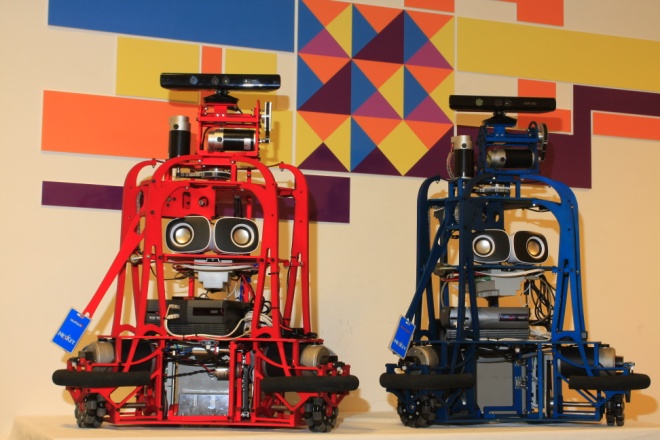
- 1.10. Ethon robots and the aesthetic marker concept
- 2.1. Main use cases of robot middleware
- 2.2. The graphical interface of RTC Builder
- 2.3. The architecture of RT component
- 2.4. The graphical interface of the System Editor of the OpenRTM-aist
- 3.1. The block diagram of the joint controller RTC
- 3.2. Block diagram of the 3 axis CNC controller
- 3.3. Default (a) graphical user interface of LinuxCNC software system
- 3.4. Customized (b) graphical user interface of LinuxCNC software system
- 3.5. (a) Typical system layout of the LinuxCNC based motion controller
- 3.6. (b) Typical system layout of the LinuxCNC based motion controller
- 3.7. RS485 expansion (a) bus
- 3.8. RS485 expansion (b) module concepts
- 3.9. Examples of (a) analogue incremental servo interface
- 3.10. Examples of (b) differential incremental servo interface
- 3.11. Mechanical drawing of the Adept 604-S SCARA robot. m1, m2, m3 are the masses, l1,l2,d0,d3 are the length, q1,q2,q3,q4 are the angles of the corresponding joints. (These data are necessary only for the calculations of robot dynamics: lc1 and lc2 are the masses position on joint 1 and joint 2, respectively.)
- 3.12. Shows (a) control of the modular controller
- 3.13. Shows (b) power amplifier of the modular controller
- 3.14. Shows (c) power electronics shelves of the modular controller
- 4.1. Information streams of the Telemanipulation (adapted from [3])
- 4.2. General concept of the telemanipulation
- 4.3. Ideal Telepresence systems: (a) Revolute motion manipulation, (b) Linear motion manipulation
- 4.4. Layer definition for the general concept of the Internet-based Telemanipulation.
- 4.5. Sensor Layer definition for the general concept of the Internet-based Telemanipulation.
- 4.6. Manipulator Layer definition for the general concept of the Internet-based Telemanipulation.
- 4.7. Layer definition for the general concept of the Internet-based Telemanipulation
- 4.8. Telemanipulation in the virtual reality
- 4.9. Micro/nano teleoperation system
- 4.10. A point type master device
- 4.11. An arm type master device
- 4.12. A glove type master device
- 4.13. Mechanical structure of the sensor glove
- 4.14. Finger movement in the glove
- 4.15. Structure of one D.O.F. of the Sensor Glove
- 4.16. Concept of the Micro Telemanipulation
- 4.17. The photo of the Master Device
- 4.18. The photo of the Slave Device
- 4.19. Object Grasped by 3 Fingers
- 4.20. Contact Point and Contact Frame
- 4.21. Conventional bilateral control schema with force and position feedback
- 4.22. Conventional bilateral control schema with two position control loops
- 4.23. The Configuration of the Smith Predictor
- 4.24. A simple teleoperator with time delay Td.
- 4.25. Telemanipulation with wave variables
- 4.26. Sliding mode based feedback compensation
- 4.27. Discrete-time chattering phenomenon
- 4.28. Controller scheme for position control
- 4.29. Experimental results: Position control tests
- 4.30. Overall control scheme for force control
- 4.31. Experimental results of one joint of glove type device; (left) PID, (right) PID with disturbance observer, angel of motor, torque of human joint, output voltage and estimated disturbance
- 4.32. The geometry setup of wirtual wall touching experiment
- 4.33. Meassurement results of virtual wall touching, depth from the operator’s palm (upper) and the torque (middle)
- 4.34. Visual feedback for the operator
- 4.35. Classical MRAC scheme
- 4.36. Sliding mode based MRAC scheme
- 4.37. Axis X: Comparison of the response of the reference model and the real plant
- 4.38. Axis Y: Comparison of the response of the reference model and the real plant
- 4.39. Tele Handshaking Device: (a) Photo (b) Structure
- 4.40. One DOF linear motion manipulator with virtual impedance
- 4.41. Virtual Impedance with Position Error Correction for a teleoperator system with time delay
- 4.42. Control diagram the Handshaking device
- 4.43. Experimental results of tele handshaking device without time delay (a) Results with VI and without PEC
- 4.44. Experimental results of tele handshaking device without time delay (b) Results with VIPEC
- 4.45. Experimental results of tele handshaking device with 400 ms time delay (a) Results with VI and without PEC
- 4.46. Experimental results of tele handshaking device with 400 ms time delay (b) Results with VIPEC
- 5.1. MogiRobi: the holonomic drive based ethological robot
- 5.2. The concept of the iSPACE and the behaviour attitude
- 5.3. MogiRobi expressing sadness
- 5.4. MogiRobi expressing happiness
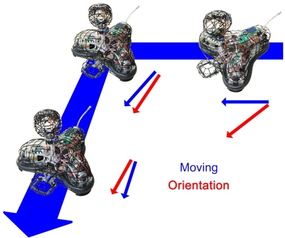
- 5.5. Different direction of moving and looking during holonomic movement.
- 5.6. The basement of the robot
- 5.7. The design of the basement
- 5.8. The omnidirectional wheels
- 5.9. The neck of the robot
- 5.10. The ball joint of the head
- 5.11. The head
- 5.12. The gripper
- 5.13. The oscillating mechanical system and the wired servo drive
- 5.14. The tail
- 5.15. The motion control board
- 5.16. The servo control board
- 5.17. The LCD and the control buttons
- 6.1. Diagram of the fuzzy automaton
- 6.2. FRI based Fuzzy Automaton.
- 6.3. FRI behaviour-based structure
- 6.4. Structure of the simulation
- 6.5. Screenshot of the simulation application
- 6.6. A sample track induced by the exploration behaviour component
- 6.7. A sample track induced by the ‘DogGoesToDoor’ behaviour component
- 6.8. Some of the state changes during the sample run introduced in
- 6.9. Fuzzy partition of the following terms: dgro - dog greets owner, dpmo - dog’s playing mood with the owner, dpms - dog’s playing mood with the stranger, dgtt - dog goes to toy, dgtd - dog goes to door, oir - owner is inside, ogo - owner is going outside
- 6.10. Fuzzy partition of the term ddo (distance between dog and owner)
- 6.11. Fuzzy partition of the term danl (dog’s anxiety level)
- 6.12. Fuzzy partition of the term dgto (dog is going to owner) and dgtd (dog is going to the door)
- 8.1. Leonardo da Vinci’s studies about the influence of apparent area upon the force of friction.
- 8.2. Amonton’s sketch of his apparatus used for friction measurement in 1699.
- 8.3. Contact surfaces at microscopic level
- 8.4. Visualization of rigid bodies in contact
- 8.5. The breaking of bristles
- 8.6. Coulomb friction characteristic
- 8.7. Viscous friction combined with Coulomb friction
- 8.8. Viscous friction combined with Coulomb friction and static friction
- 8.9. Stribeck friction characteristic
- 8.10. Steady state friction-velocity curve used for simulation
- 8.11. Karnopp model, stick-slip curve
- 8.12. Seven-parameters model, stick-slip curve
- 8.13. LuGrell model, stick-slip curve
- 8.14. Modified Dahl model, stick-slip curve
- 8.15. M2 model, stick-slip curve
- 8.16. Seven-parameters model, change of friction force during velocity reversals
- 8.17. Seven-parameters model, change of spring force during velocity reversals
- 8.18. Seven parameter model, change of mass velocity during velocity reversals
- 8.19. Seven parameter model, change of displacement during velocity reversals
- 8.20. Dahl model, change of spring force during velocity reversals
- 8.21. Modified Dahl model, change of mass velocity during velocity reversals
- 8.22. Modified Dahl model, change of displacement during velocity reversals
- 8.23. Modified Dahl model, change of displacement during velocity reve
- 8.24. LuGre model, change of spring force during velocity reversals
- 8.25. LuGre model, change of mass velocity during velocity reversals
- 8.26. LuGre model, change of mass displacement during velocity reversals
- 8.27. LuGre model, change of friction force during velocity reversals
- 8.28. Karnopp model, change of mass velocity during velocity reversals
- 8.29. Karnopp model, change of mass displacement during velocity reversals
- 8.30. Karnopp model, change of friction force during velocity reversals
- 8.31. Karnopp model, change of spring force during velocity reversals
- 8.32. M2 model, change of mass velocity during velocity reversals
- 8.33. M2 model, change of mass displacement during velocity reversals
- 8.34. M2 model, change of friction force during velocity reversals
- 8.35. M2 model, change of spring force during velocity reversals
- 8.36. Presliding displacement curve of the seven-parameters friction model
- 8.37. Presliding displacement curve of LuGre model
- 8.38. Presliding displacement curve of Modified Dahl model
- 8.39. Presliding displacement curve of M2 model
- 9.1. Connection layout of PCI card based motion control system
- 10.1. PCI card connectors and LEDs
- 10.2. Pin numbering of RS485-bus connector
- 10.3. Pinout of RS485-bus connector
- 10.4. Equivalent circuit of an output pin. Direction of I/O pins depending on configuration see chapter 4.9
- 10.5. Pin numbering of CAN-bus connector
- 10.6. Pinout of CAN-bus connector
- 10.7. Pin numbering of axis connectors
- 10.8. Pinout of axis connectors
- 10.9. Equivalent circuit of fault input for an axis
- 10.10. Equivalent circuit of enabled outputs
- 10.11. Equivalent circuit of output pins (Step, Direction, and DAC serial line) on axis connectors
- 10.12. Pin numbering of homing & end switch connector
- 10.13. Pinout of homing & end switch connector
- 10.14. Equivalent circuit of input pins
- 10.15. Mechanical dimension
- 10.16. Axis interface modules: Differential line driver, Digital to analogue converter, Optical isolator, Encoder/ reference breakout
- 10.17. Analogue system with encoder feedback
- 10.18. Incremental digital system with encoder feedback and differential output
- 10.19. Incremental digital system with encoder feedback and TTL output
- 10.20. Incremental digital system with differential output
- 10.21. Incremental digital system with TTL output
- 10.22. Absolute digital (CAN based) system
- 10.23. Absolute digital (CAN based) system with conventional (A/B/I) encoder feedback
- 10.24. Block diagram of the optical isolator module connection
- 10.25. Pinout of PCI card (RJ50) connector and power input terminals
- 10.26. Pinout of reference output and encoder input connectors
- 10.27. Equivalent circuit of output pins
- 10.28. Fault signal input equivalent circuit
- 10.29. PCI card (RJ50) input equivalent circuit
- 10.30. RJ50 to PCI card: Fault output equivalent circuit
- 10.31. Block diagram of the digital to analogue converter module connection
- 10.32. Controller side pinout
- 10.33. Machine side pinout
- 10.34. Equivalent circuit of fault signal output
- 10.35. Enable output
- 10.36. Equivalent circuit of fault input circuit
- 10.37. Fault management flowchart
- 10.38. Block diagram of the differential line driver module connection
- 10.39. Controller side pinout
- 10.40. Machine side pinout
- 10.41. Optocoupler
- 10.42. Fault input circuit equivalent circuit
- 10.43. Block diagram of the breakout module connection
- 10.44. Pin numbering of RJ50 and RJ45 modular connectors
- 10.45. Encoder pinout
- 10.46. Encoder pinout
- 10.47. Terminal connector pinout
- 12.1. Step/Dir type reference
- 12.2. Up/Down count (CW/CCW) reference
- 12.3. Quadrant (A/B) type reference
- 13.1. 8-channel relay output module
- 13.2. 8-channel digital input module
- 13.3. 8 channel ADC and 4-channel DAC module
- 13.4. Teach Pendant module
- 13.5. Powering of the nodes
- 13.6. Bus setting
- 13.7. Connecting of the nodes
- 13.8. Node NBC addressing
- 13.9. Relay output module
- 13.10. Numbering of output terminal connector and 24 input
- 13.11. Output connection diagram
- 13.12. Pin assignment table: NO: Normally Open, NC: Normally Closed, COM: Common
- 13.13. Digital input module
- 13.14. Equivalent circuit of digital input lines
- 13.15. Numbering of input terminal connector
- 13.16. Pin assignment table
- 13.17. AD & DC modul
- 13.18. Numbering of the terminal connector
- 13.19. Pin assignment table
- 13.20. Teach pendant module
- 13.21. Connectors and pin numbering of the teach pendant module
- 13.22. Pin assignment table of the digital input connector
- 13.23. Mechanical dimensions
- 13.24. (http://grabcad.com/library/robot-puma-560) Download: 2013. november 2.
- 13.25. Blockdiagram of the control
- 13.26. Connection of the robot and of the control
Chapter 1. Introduction: Trends in robotics
According to the report of Japanese Ministry of Economics and Trade [1] the robot industry market will be rearranged dramatically (see 11. ábra). The dominance will be shifted from the classical industrial robots used in the manufacturing sector to the so called service robots, which have already overtaken the leadership in the scientific journals and conferences but his market segment was almost ignorable. It will be increased most rapidly in the near future. This perception shows the increasing trend office, hospital, and similar robots. (In most of the cases these are mobile robots.)
![Robot industry market projections [1]](images/image_0.png)
Until now, the ordinary people could see robots only in the TV but there was no real physical contact with them. It means that robots were pure engineering stuff. The engineers used them. It is unequivocal that industrial robots are used and programmed by robot specialist engineers. As the robot appearing in small and middle size enterprises the robots are handled by engineers, who are not specialized in robotics. Thus the efficiency of robot programming methods must be improved in order to avoid losses caused by frequent switches in small scale production. So there is an increasing need to make the training of robots more automatized and at the same time to make them be able to fulfill more and more sophisticated tasks.
For automated material handling an industrial robot is a very handy solution, however it needs special attention in programming of work tasks. Offline programming of industrial robot is difficult because it relies on very accurate system setups and the virtual programming environment must be carefully calibrated to capture the real-life setup and to avoid any changes of the robot program on the spot itself. These problems could be avoided by using online programming of principles, but during online programming the robot is unable to produce anything. This results a continuous demand for new and effective robot teaching methods. In the field of industrial robotics the most challenging obstacle is that it takes approximately 400 times longer to program an industrial robot in complex operations than to execute the actual task [2].
In the next step the robot will be used by non engineers. In the aspect of robot users people can be divided to 4 main groups.
robot specialist engineer
engineer, but not robot specialist
not engineer, but being interested in robotics
elderly people, reluctant to robotics
For robots in our daily life it is not enough to execute a pre-programmed action line. They must be able to adopt themselves to changing environment, make their own decisions and in addition, they have to socially fit into the human environment. This requires a more sophisticated robot control method. The way of usage must be as simple (or simpler) as the usage of every office, or household devices. Service robots are designed for more sophisticated tasks than other devices, so the robot control method and the artificial intelligence must satisfy the communication tasks at a human-robot interaction. In line with the hardware design, the low level software development this train of thought raises several additional questions like
How should a social robot look like?
How should we communicate with the robot?
Is it possible for a robot to have emotions?
What is the definition of emotions?
People have always felt attached to their articles for personal use (phone, car, etc.). This attachment can be stronger to service robots. Turning this - currently unilateral attachment relationship - into a mutual relationship can bring not only obvious marketing advantages but enhance cooperative effectiveness in human-system interactions
1.1. Human Robot Cooperation on shopfloors
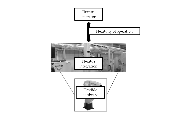
While service robots are about to infiltrate everyday life still a significant effort is given to the research of robotic manipulators. As service robots become friendlier and more natural the underdevelopment of operation and programming possibilities of a manipulator becomes clear. Since small and medium enterprises (SMEs) are turning to automation the need for flexible robot cell integration is rising. Flexibility may depend on several factors:
Hardware flexibility (robot, CNC machine)
Integration flexibility (reconfiguration of robot cell)
Operation flexibility(human robot interaction)
The first two components are addressed my both the robot manufacturers and informatics technology researches. The main challenge on this field is to provide a standard protocol for the different components building up the whole production system. The service oriented architecture (SOA) paradigm [3] offers a scientifically accepted approach and it is still in the main flow of interest [4, 5, 6].
On the other hand the least flexible point of a whole system defines its overall flexibility. The problem is well defined in [7]: most flexible robot cells are sold with custom operating software and as a result the key to operational flexibility remains in the hands of the integrator. To bring more adaptively in operation [7] presents a set of robust control software. Furthermore one has to keep in mind that SMEs are often not in the position to employ highly trained operational personnel thus the easy programming and configuration contribute to flexibility (see 12. ábra). Human robot cooperation is still in the focus because of the goal for simple robot programming.
1.1.1. Robot operation in shared space
The easiest and most natural way of programming a robot is to teach the task by hand. Moving the manipulator by hand implies danger: the robot should be energized thus a robust and safe control system is needed. Any autonomous movement of the manipulator is potentially dangerous when humans must stay or work in the reach of the robot. Controlling the human robot interaction force offers a solution and implementing impedance control [8] with use of force sensor showed feasibility of collaboration without fences. Another control scheme is presented by [9] with the comparison of PD and sliding mode controller algorithms.
The other possibility to overcome this issue is to develop compliant robot systems. The lack of robustness in previous systems prompted research for new technology. [10] Presented a control system for manipulator actuated by pneumatic muscles while [11] and [12] uses direct-drive motors with wire rope mechanism.
The trend in industrial manipulator control research points clearly towards robust but compliant systems to merge accuracy and safety.
1.1.2. Flexible human robot interaction
In the framework of human robot cooperation the most important aspect is the bilateral communication. Physical interactions carry safety problems mentioned in the previous sub-section and environment awareness of the robot is still a significant problem. The more effective and flexible interaction with the user is intended the more sophisticated recognition technology is required.
Interesting example is presented by [13]. With traditional approach an additional channel should be used to communicate information about the object handed to the robot by the user. The use of a tactile sensor gives better potential for the robot system to understand the human intentions thus expanding the modularity of the interaction.
From the operators point of view better understanding of the system is possible to realize through user interfaces adapted to various contributors:
Complexity of the robot cell
Complexity of the task performed by the robot cell
Competence of the operator
Information needed
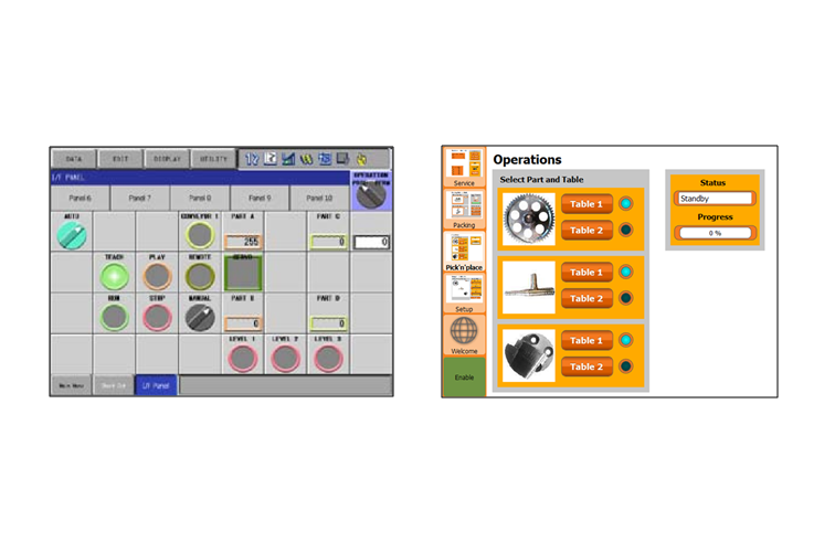
The key toward better flexibility is to transform the traditional and very technical graphical user interfaces between humans and industrial robots (see 1-3. figure). The focus should be shifted from the practical operation of a robot cell towards the cognitive programming and operation. Research on this includes other fields like psychology, usability, human factors.
Traditionally industrial robots are machines with as minimal human interaction as possible. Including the human in the operation not only increases the flexibility and efficiency but brings improved understanding in human robot relations and takes a new step toward better trust in automation in overall.
1.2. Engineering concepts for service robotics
Robots at the service sectors have to fulfill more and more sophisticated tasks. This is the same trend like at the evolution of industrial robots. The first industrial robot was created in 1937 by Griffith P. Taylor. [14] It contained almost only mechanical parts, and only one electric motor. It could stack wooden blocks in pre-programmed patterns. The program was on a punched paper, which activated solenoids. Nowadays industrial robots can weld, paint, mill, etc.
In a point of view the simplest robots at home are the washing machines, blenders, dishwashers, etc. These devices are created to help our daily routine tasks. The next step of this evolution is the help at our daily service type tasks. Inherently from the service tasks most of the robots in the service sector are mobile robots.
There are several responsive robot platforms can be found for to help us somehow, or simply just for fun. Roomba [15], or Navibot [16] helps to clean up the household in simple and convenient way like never before. There are also some doglike equipment like AIBO [17], or Genibo but these items are just trying to act as a real dog in a very primitive level. Some human inspired robots are also available, like Honda's ASIMO [18], or SONY's QRIO [19], but these complex and technically very advanced platforms are also just scratching the surface of the real social interaction between machine and human.
For the elders there is Paro [20] or Kobie, a kinds of a therapy robots, which are capable to perceive light, sound, temperature and touch, thus they are capable to sense their environment and the surrounding people. These robots could interact with the user in simple ways. They could learn the preferences of the elder in behavior, and react to their names. Even “simple” toys like these could reduce the stress level of the user, help to increase the socialization between the elders and make the communications with the caregivers more flawless.
1.2.1. Movement of the robots
Several types of mobile robots exists like tracked, wheeled, legged, wheeled-legged, leg-wheeled, segmented, climbing or hopping. The control methods of these robots are implemented individually for every construction. In most of the cases the control algorithms uses the virtual center of motion method. The path of the motion describes the path of this point [21], [22]. We can consider the whole mobile robot as a point (the centre of gravity, virtual center of motion). The velocity and the angular velocity of the centre of gravity define the motion of the robot (at constant speed). At the path of the motion we prescribe the velocity and the angular velocity of the robot in every moment.
The most often ways for mobile robot motion are the differential type drive and the steered vehicle concept. The path planning of these mechanical constructions can be extremely difficult [23]. Indoor environments increase the number of questions in this method. (see in 14. ábra)
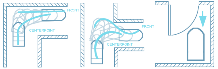
At different driven type mobile robots path planning is simpler, because the robot can turn around without the change of the position. The orientation of the robot is always the same with the moving direction. These robots (and the driven vehicles also) have only 2 DoF-s on the ground plane.
In 1994 Stephen Killough invented omni wheels. [24] These are wheels with small discs around the circumference which are perpendicular to the rolling direction. This type of wheel does not have a geometrical constrain perpendicular to the rolling direction. With this type of configuration we can get a 3 DoF holonomic system (x, y, rot z). The most of the overland animals can move in 3DoF: turning and moving in one direction in the same time. The ordinary drive systems (steered wheels, differential drive) cannot perform this.
1.2.2. Informatics concepts
The artificial intelligence of a service robot system can be implemented on the robot, or distributed between the robot and the external environment (Intelligent Space). The Intelligent Space (iSpace) is an intelligent environment which provides both information and physical supports to humans and robots in order to enhance their performances. In order to observe the dynamic environment, many intelligent devices, which are called Distributed Intelligent Network Devices, are installed in the iSpace. [25, 26]
At the current state of science the greatest problem is caused by self-localization of robots (orientation, obstacle avoidance, path planning, etc.). There are several types of sophisticated methods for this problem. [27]
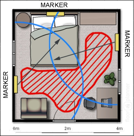
Could they be moved without requiring our presence? [28] Optical markers are generally developed for this kind of positioning. [29] (15. ábra) The most generally know optical marker is the QR code. QR code is designed only with the consideration of visual recognition and redundant information storage. (16. ábra)

1.3. Etho-Robotics
Ethology will play a major role in future development of social robotics because the emergence of new robotic agents does not only pose technological questions [30]. Only a broad synergic view of biological causality (ultimate and proximate), which has been practiced in ethology for at least half a century [31], can provide the necessary theoretical network which is able to handle future challenges.
May be a recent analogy could help in revealing our intentions with regard to social robotics. [32], investigated the head structures of woodpeckers in order to find out how the woodpecker’s head is protected against the vibration caused by drumming behaviour. The motion of a biological being has communication related senses.
According to human evolution we, can usually recognize the purpose, the behavior and the mood of an animal. The goal is to enhance the artificial devices with this natural interoperability, creating a way of human-machine interactions which stands for human needs. Instead of specifying any improvised implementation based on individual intuitions, the characteristics of the etho-inspired machine behavior has to be defined with a standardized methodology. These definitions are relying on organized observations of the natural behaviors, with a collection of perceptions. During the pre-organization of these tests, the observed and analyzed behavioral variables have to be defined those can make any sense for a human witness in a given scene and situation. As in many disciplines, the tests have to be performed with many subjective individuals for getting an objective result. The analyzing method consists of two simple steps: For first, the impressions and potential lateral information should be collected, which caused by the main character of the test situation. Then the impressions and information have to be conjugated to the behavioral variables in a systematic way, which allows a weighted overlap between the nodes. The weight factors must be given by using the statistics of the many performed observations.
An illustrative example, when a predator animal runs for a specified target (position) in a non-straight trajectory, because of an interfering obstacle. The most of the observers can conclude the goal position while the direction of the run is not pointing to the target. Here, the essential behavioral variable is the looking direction which contains the lateral information.
Using these analyzed measurements, a fuzzy model can be created that implements the initial concept. In many cases, the implementations require the use of new technologies. The solution of the animal like locomotion with different looking direction, body orientation and moving direction was induced the usage of holonomic robot platforms. 17. ábrashows the above example scene, where the implemented solution can be validated by repeating the observation tests with the robot, concluding that the lateral information is reflected by the behavior.
1.3.1. Informatics concepts with etho-inspiration
The best concept for the artificial intelligence is to use the abstract ethological model of the 20,000 year old human-dog relationship as the basis for the human-computing system interaction. [6] The mathematical description of the dog’s attachment behavior towards its owner is an essential aspect of setting up the ethological communication model. Such approach needed an interaction among various scientific
disciplines including psychology, cognitive science, social sciences, artificial intelligence, computer science and robotics. The main goal has to find ways in which humans can interact with these systems in a “natural” way.
These systems do not have emotions, but they can act in a way that makes us believe that they are actually fond of us. While there is a need for a mathematical model of the system, the complexity of the applied solution must fit the complexity of the problem. In case of neural networks it concerns the number of the neurons and connections, in case of fuzzy logic system; there is a minimal value of the number of the fuzzy sets and fuzzy rules. Since elderly people are naturally mistrustful toward new technologies, a solution like this could makes easier to use the modern devices and fell the interactions more natural. A device like this could substitute assistant dogs in some special situations, or could cooperate with the pets to serve the elderly people in need.
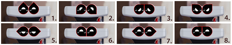
As it mentioned in the previous section markers are used for robot localization. Existing markers were designed to be practical and not aesthetic, thus people did not welcome them in their homes. Who would want the walls of their home or work place to be filled with QR codes? Aesthetical appearance depends on proportional harmonization of composition, tone, pattern and rhythm. Through aesthetics marker design the goal is to create harmony between human visual recognition and image processing of robots. [29] (see 18. ábra) Without appropriate engineering methods and devices the information science would not be sufficient to express emotions. As it mentioned in section 1.2.1, the holonomic movement is one of these etho-inspired engineering methods. The eyes of the robot are especially important at the expression of emotions. (see 19. ábra) With the use of basic geometrical shapes, colors and arrangements basic emotion can be recognized.
1.4. Conclusion for the introduction
Often machines can replace humans for more effective manufacturing because machines outperform humans in terms of strength, precision and endurance. Humans, however, perform better than machines when flexibility and intelligence is required.
![Aesthetic markers, [10]](images/image_8.png)
This paper shows efficient methods and processes for teaching and optimizing complex robot tasks by introducing etho-robotics and flexible robotics. Intelligent user interfaces combining information from several sensors in the manufacturing system will provide the operator with direct knowledge on the state of the manufacturing operation. Thus, the operator will be able to determine the system state quicker. Sensory system calculates and proposes the optimal process settings. The key element is the new human-machine communication channels helping the human to comprehend the information from the sensory systems.
1.5. References for Robotics trends
[1] Ministry of Economics and Trade (METI). (2010). 2035nen ni muketa robotto sangyou no shourai shijou yosoku (Market forecast of robot industry in 2035). Retrieved: http://www.meti.go.jp/press/20100423003/20100423003-2.pdf
[2] T. Thomessen, P. K. Sannæs, and T. K. Lien, “Intuitive Robot Programming,” in Proc. 35th International Symposium on Robotics, 2004.
[3] F. Jammes, H. Smit, "Service-oriented Paradigms in Industrial Automation" IEEE Trans. on Industrial Informatics, vol. 1, no. 1, pp. , Feb 2005.,
[4] G. Candido, A.W. Colombo, J. Barata, F. Jammes, "Service-Oriented Infrastructure to Support the Deployment of Evolvable Production Systems" IEEE Trans. on Industrial Informatics, vol. 7, no. 4, pp. 759 - 767 , Nov 2011.
[5] R. Kyusakov, J. Eliasson, J. Delsing, J. van Deventer, J. Gustafsson, "Integration of Wireless Sensor and Actuator Nodes With IT Infrastructure Using Service-Oriented Architecture" IEEE Trans. on Industrial Informatics, vol. 9, no. 1, pp. 43-51, Feb 2013.
[6] M. GarciaValls, I.R. Lopez, L.F. Villar, "iLAND: An Enhanced Middleware for Real-Time Reconfiguration of Service Oriented Distributed Real-Time Systems" IEEE Trans. on Industrial Informatics, vol. 9, no. 1, pp. 228-236, Feb 2013.
[7] A. Ferrolho, M. Crisostomo, "Intelligent Control and Integration Software for Flexible Manufacturing Cells ," IEEE Trans. on Industrial Informatics, vol. 3, no. 1, pp. 3-11, Feb 2007.
[8] G. Ferretti, G. Magnani, and P. Rocco, “Impedance Control for Elastic Joints Industrial Manipulators,” IEEE Trans. Robot. Autom., vol. 20, no. 3, pp. 488–498, Jun. 2004.
[9] L.M. Capisani, A. Ferrara, "Trajectory Planning and Second-Order Sliding Mode Motion/Interaction Control for Robot Manipulators in Unknown Environments" IEEE Trans. on Industrial Electronics, vol. 59, no. 8, pp. 3189-3198, Aug 2012.
[10] Tae-Yong Choi, Ju-Jang Lee, "Control of Manipulator Using Pneumatic Muscles for Enhanced Safety ," IEEE Trans. on Industrial Electronics, vol. 57, no. 8, pp. 2815 - 2825 , August 2010.
[11] C. Mitsantisuk, S. Katsura, K. Ohishi, "Force Control of Human–Robot Interaction Using Twin Direct-Drive Motor System Based on Modal Space Design" IEEE Trans. on Industrial Electronics, vol. 57, no. 4, pp. 1383 - 1392, April 2010.
[12] C. Mitsantisuk, K. Ohishi, S. Katsura, "Control of Interaction Force of Twin Direct-Drive Motor System Using Variable Wire Rope Tension With Multisensor Integration" IEEE Trans. on Industrial Electronics, vol. 59, no. 1, pp. 498-510, Jan 2012.
[13] K. Suwanratchatamanee, M. Matsumoto, S. Hashimoto, "Robotic Tactile Sensor System and Applications ," IEEE Trans. on Industrial Electronics, vol. 57, no. 3, pp. 1074 - 1087 , March 2010.
[14] Griffith P. Taylor, "An Automatic Block-Setting Crane". Meccano Magazine (Liverpool UK: Meccano) 23 (3): 172. March 1938.
[15] Jone J.L., “Robots at the tipping point: the road to iRobot Roomba”, IEEE Robotics & Automation Magazine, Vol. 13, Issue 1, pp. 76-78, Marc. 2006.
[16] Eric Guizzo, “Robot Vacuums That Empty Themselves”, IEEE Spectrum, 16. Jan. 2012.
[17] Fujita M. “On activating human communications with pet-type robot AIBO”, Proceedings of the IEEE, Vol. 92, Issue 11, Nov. 2004.
[18] Sakagami Y, Watanabe R, Aoyama C, Matsunaga S, Higaki N, Fujimura K, “The intelligent ASIMO: system overview and integration”, Intelligent Robots and Systems, Vol. 3, pp. 2478-2483, 2002,
[19] Tanaka F, Suzuki H, “Dance interaction with QRIO: a case study for non-boring interaction using an entrainment ensemble model”, Robot and Human Interactive communication, pp. 519-424, 2004.
[20] Shibata T, Kawaguchi Y, Wada K, “Investigation on living people with Paro at home”, Robot and Human Interactive Communication, pp. 1131-1136, Toyama, 2009.
[21] Martin Udengaard, Karl Iagnemma, “Kinematic Analysis and Control of an Omnidirectional Mobile Robot in Rough Terrain” in Intelligent Robots and Systems, San Diego, pp. 795-800, 2007.
[22] H. Adachi, N. Koyachi, T. Arai, A. Shimizu, Y. Nogami, “Mechanism and Control of a Leg-Wheel Hybrid Mobile Robot” in International Conference on Intelligent Robots and Systems, Kyongju, pp. 1792-1797, 1999.
[23] S.A. Arogeti, Danwei Wang, Chang Boon Low, Ming Yu, " Fault Detection Isolation and Estimation in a Vehicle Steering System ," IEEE Trans. on Industrial Electronics, vol. 59, no. 12, pp. 4810-4820, Dec 2012.
[24] Stephen Killough, "1997 Discover Awards". Discover Magazine, Retrieved 22, September 2011.
[25] Kovács B., Szayer G., Tajti F., Korondi P. Nagy I., "Robot with Dog Type Behaviour", EDPE 2011, pp. 4, 5
[26] QinZhang,L. Lapierre, XianboXiang " Distributed Control of Coordinated Path Tracking for Networked Nonholonomic Mobile Vehicles ," IEEE Trans. on Industrial Informatics, vol. 9, no. 1, pp. 472-484, Feb 2013.
[27] D. Lee, W. Chung, "Discrete-Status-Based Localization for Indoor Service Robots," IEEE Trans. on Industrial Electronics, vol. 53, no. 5, pp. 1737-1746, Oct 2006.
[28] W. Chung, S. Kim, M. Choi, J. Choi, H. Kim, C. Moon, J.-B. Song, "Safe Navigation of a Mobile Robot Considering Visibility of Environm," IEEE Trans. on Industrial Electronics, vol. 56, no. 10, pp. 3941-3950, Oct 2009.
[29] Korondi Péter, Farkas Zita, Fodor Lóránt, Illy Dániel Aesthetic Marker Design for Home Robot Localization. In: 38th Annual Conference of the IEEE Industrial Electronics Society (IECON 2012). Montreal, Kanada, 2012.10.25-2012.10.28. pp. 5510-5515.
[30] Miklósi, Á., Gácsi, M. 2012. On the utilization of social animals as a model for social robotics. Frontiers in Psychology, 3: 75
[31] Tinbergen, N (1963). On aims and methods of ethology. Zeitschrift für Tierpsychologie, 20, 410- 433.
[32] Yoon, S-H, Park S. (2011). A mechanical analysis of woodpecker drumming and its application to shock-absorbing systems. Bioinsp. Biomim. 6, 1-12.
Chapter 2. Robot middleware
The primary goal of this chapter is to find a robot framework in this environment that is easy to use, reliable and also easy to extend. After the different robot middleware concepts are detailed the most popular ones will be compared.
2.1. Introduction
RT-middleware (Robot Technology Middleware) is a technology that implements several key concepts needed for the development of complex robot systems, even in geographically distributed environments. Through a useful API, reusable standardized components and communication channels, and some degree of automatization, RT-middleware helps the user to build easily reconfigurable systems. The behavior of the components and the manner of interaction among them are standardized by the Robot Technology Component (RTC) specification. Until now there have been two implementations of the specification. OpenRTM.NET is written in .NET, while the other implementation, called OpenRTM-aist.
Within the robotics area, the task of robot systems can change quickly. If the job and environmental circumstances change frequently, reusable and reconfigurable components are needed, in addition to a framework which can handle these changes. The effort needed to develop such components depends on the programing language, the development environment and other frameworks used. Many programming languages can be applied for this process, however developing a brand new framework is a difficult task. Applying an existing framework as a base system, such as the OpenRTM-aist in the case of this chapter, the associated development tasks can be dramatically simplified.
Frameworks and middleware are gaining popularity through their rich set of features which support the development of complex systems. Joining together any robot framework and robot drivers can form a complex and efficient system with relatively small effort. In many cases, the task of the system designer is reduced to the configuration of an already existing framework.
On the other hand, when an existing framework requires only a set of completely new features, it can simply be extended with them. Improving an existing framework is an easier job than developing a new one because the design and implementation of such a system requires specialized knowledge and skills (design and implementation patterns). In most cases, the missing functionalities can be simply embedded into the existing framework, nonetheless there are some cases when this is hard to achieve. An existing framework can be improved simply only in case it is well designed and implemented. In spite of this, building a brand new system from is a much longer process that requires much effort.
In the area of robotics, there are many robot parts that share similar features, so the concept of robot middleware as a common framework for complex robot systems is obvious. Probably there is no framework which can fulfill all of the above requirements entirely.
2.2. Requirements of the robot middleware
In this section, I explore the requirements of robot middleware technologies in general and examine some existing robot approaches such as YARP, OpenRDK, OpenRTM-aist and ROS.
Robot middleware is a software middleware that extends communication middleware such as CORBA or ICE. It provides tools, libraries, APIs and guidelines to support the creation and operation of both robot components and robot systems. Robot middleware also acts as a glue that establishes a connection among robot parts in transparent way.
First of all, we should define the requirements and the actors of robot middleware. Generally, two actors use such technology: end-users and developers. Every robot middleware has to provide tools and mechanisms to facilitate the work of these actors.
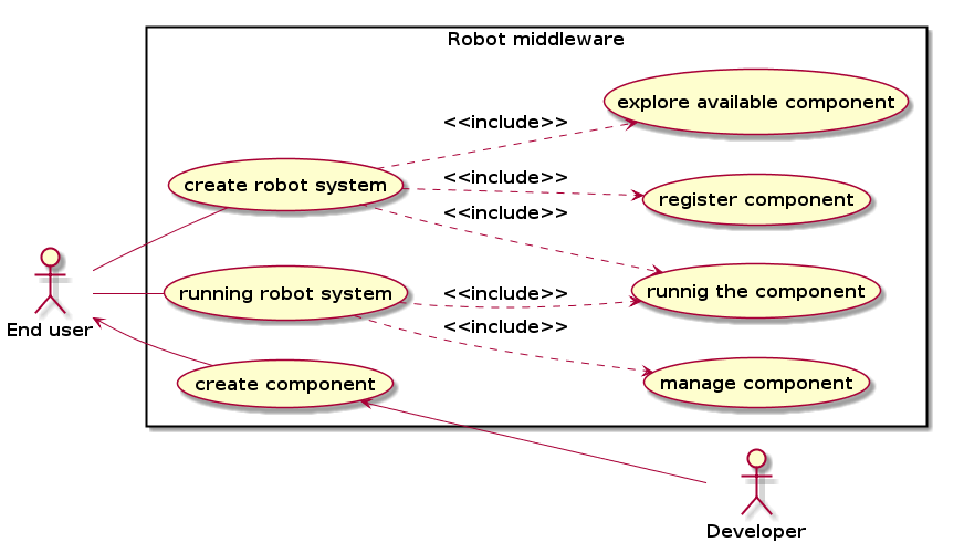
The main use cases of robot middleware are shown in 21. ábra. After the analysis of these use case we can define some functional requirements. The component developers design and implement components. For this development procedure, many programming languages and operating systems should ideally be supported. Tools are needed for the generation of skeletons and semi-working components for quicker development. The main activity of the developer actor should be the generation of semi code, the filling out of business logic, the compilation of binary code and the execution of test cases. Developers also create robot parts as components using their knowledge about programming languages, robot middleware and the specification of the given robot system. Moreover, the person who develops the component has to validate it as an end-user. In summary, from the developer's point of view, the main requirements for robot middleware are as follows:
Support for a variety of programming languages: in most cases the members of research and development teams who develop various robot parts will be familiar with different languages depending on the trend at any given time.
Support for a variety of operating systems: nowadays Windows and Linux operating system support is mandatory, as heterogeneous systems may rely on other libraries as well that are specific to these systems.
Skeleton generation and other tools for components: The framework should be able to generate skeleton code for component development in order to speed up the development process. For this reason, robot middleware technology should include templates and tools (preferably graphical tools) to aid component development. Although developers will have to learn how to use the tools to generate source code, this requires less effort than starting component development from the scratch.
As opposed to the developer actor, an end-user is someone who has no knowledge about programming languages, as is not interested in developing components. End-users simply want to use components for their own work. In their case only a minimum number of system parameters should be visible, which are sufficient for the creation and operation of the robot system. Nice graphical interfaces and visual aid features are useful to end-users in allowing for the straightforward operation of the robot system. End-users have two main tasks. First, they often create complex robot systems using existing robot parts, and second, they often want to run previously created robot systems. The creation of a robot system can include a search for available robot parts during which the user obtains information about the accessibility of available components. This accessibility information can depend on the specific robot middleware which is applied for the task, and may include IP numbers, or any internal identifiers or symbolic names. Unfortunately, most robot middleware systems only support online components. For this reason, robot parts have to be available during the robot system creation process, i.e. have to be already running and must be registered.
End-users want to register their components in order to share functionalities with other end-users. After registration, the component can be found by all other participants. Usually end-users create custom robot systems using available components, so the second task is to find out which of the components are running. Once the robot systems are running, users will want to control them, i.e. activate/deactivate any or all of the components, and run them with various different parameter sets.
In summary, from the end-user point of view, the main requirements for robot middleware are as follows:
The overall change in the applications and general software components running on workstations in a research group should be minimal. In most cases the operation of any system that is relied on by end-users on a daily basis requires a special software environment. The installation of new software components may result in outage periods in terms of existing services.
User-friendly graphical interface the graphical interface of robot middleware should be as user-friendly as possible.
Like developers, end-users would like to use Windows or Linux systems, therefore Windows and Linux operating system support is a strong requirement. End-users will not replace their familiar workstation environment with a new one just to accommodate the requirements of a new robot middleware.
In summary, the key consideration for a robotics middleware system to be useful is that it should provide an efficient API and as much automatization as possible. Additionally, middleware systems also have to support as many operating systems and programing languages as possible. If a framework is applied for a specific task, some efforts will always be needed to understand the relevant concepts and application details.
2.3. Existing robot middleware
One distributed environment for robot cooperation is OpenRDK. The concept is detailed by Calisi in [1] . The user’s robot system can be developed using a set of Agents, through a simple process. A Module is a single thread inside an agent process. Every module has a repository in which a set of internal properties are published. Inter-agent (i.e., inter-process) communication is accomplished by two methods: through property sharing and message sending. RConsole is a graphical tool for remote inspection and management of modules. It can be used as both the main control interface of the robot and for debugging while developing software. It is just an agent that happens to have some module that displays a GUI. The framework can be downloaded from [2] .
Alternative important robot middleware platform is Yet Another Robot Platform (YARP). Communication in YARP generally follows the Observer design pattern (for more details see [3] ). Every YARP connection has a specific type of carrier associated with it (e.g., TCP, UDP, MCAST (multi-cast), shared memory, within-process). Ports can be protected by SHA256 based authentication. Each port is assigned a unique name and it is registered into a name server. The YARP name server, which is a special YARP port, maintains a set of records, the keys of which are text strings (the names of the ports). The remainder of each record contains whatever information is needed to make an initial connection to a given port.
The third important robot middleware technology is OpenRTM-aist (documentation about it can be found [4] ), which is a convenient modular system also built on the Common Object Request Broker Architecture (CORBA). This concept uses the distributed components approach, where the components have to be registered into central naming service. (The openRTM-aist uses the name server of CORBA system.). The whole concept is detailed by Ando et al in [5] , [6] and [7] . The components can contain modules what can be loaded any time. The framework is implemented using design patterns, robust software system, which provides huge feature set, more than previously mentioned ones. The components of robot system have same rights no central logic (except the naming service). Each RT-Component has an interface (a "port") for communication with other components. The RT system is constructed by connecting the ports of multiple components to each other in order to aggregate RT-Component functions. The advantage of OpenRTM-aist is that it provides a simple way to create and co-operate various robot parts. Two kinds of port can be used the service port and the data port. The data ports provide the asynchronous messages and the service port establishes the synchronous communication. The usage of service port is complicated because we have to know the CORBA technology that is an out of date system. The connection among components has to be established at runtime by the end-user using a graphical interface. A comfortable state machine concept is provided i.e. the developer has to override the appropriate methods only. More programing languages and mostly used operating systems are supported. This is the second popular robot framework in the world. (The most popular in Japan.)
The final investigated robot framework is the ROS (Robot Operating System), that seems a basic operating system, but it provides similar features as previously mentioned (available at [8] ). The concept is detailed by Quigley in [9] . The items of robot system have to be registered a central server as well, but this component is called ROS node in this case. This node is the basic structure that can not be divide more parts in official ROS, but a 3rd party component exists called nodelet which support run more algorithm in one process (node). A central process has to be run (one roscore file creating a ros master and rosout nodes) providing the central log opportunity and a distributed parameter set. The connections among node are established automatically, i.e. if a component is running that advertises the topic and the other which subscribe to the topic, then the two nodes store information about the other using the roscore API. The developers' work is assisted completely, but only few tools are available end-user. This is the most popular robot middleware all over the world.
In the case of all investigated robot framework a concept is handled as distributed entity that is an agent or a port or a component or a node. The YARP provides more communication possibility nevertheless it has poor set of tools. Unfortunately the development of YARP and OpenRDK is broken. Only two robot frameworks are used nowadays, the OpenRTM-aist and the ROS, which is in progress so in the later part these robot system will be compared and detailed.
2.4. Comparison of Robot middleware the point of view of developers
In this section the ROS and the OpenRTM-aist robot middleware are investigated in point of view of developer. The complexity of significant procedures are compared and additionally the helper tools.
2.4.1. Creating a new project
In the case of ROS the new package can be generated by a tool named catkin_create_package that creates a folder containing a CMakeList.txt and a package.xml. These files have to be modified if another package is needed or a new executable file is necessary. If a simple message sending or receiving is should be used then the official tutorial can be modified easily and the business logic can be placed into a single function. It doesn’t generate any file or class, but it is not necessary for usage of ROS. The structure of beginning project is very simple, understandable. The basic features of ROS can be accessed only via three classes and the implementation of business logic not requires serious knowledge of ROS system. C++ and Python programming languages are supported officially. A custom creation tool is presented called catkin_make that is an extension of the platform independent CMake build system. More Integrated Development Environment (IDE) can be used that are supported the CMake, because the CMake can export it (at the moment CodeBlocks, Eclipse, Xcode, KDevelop, and Visual Studio).
For project creation, the OpenRTM-aist middleware also contains a command line tool (rtc-template) and graphical editor, called RTC Builder (the graphical interface is shown in 22. ábra.
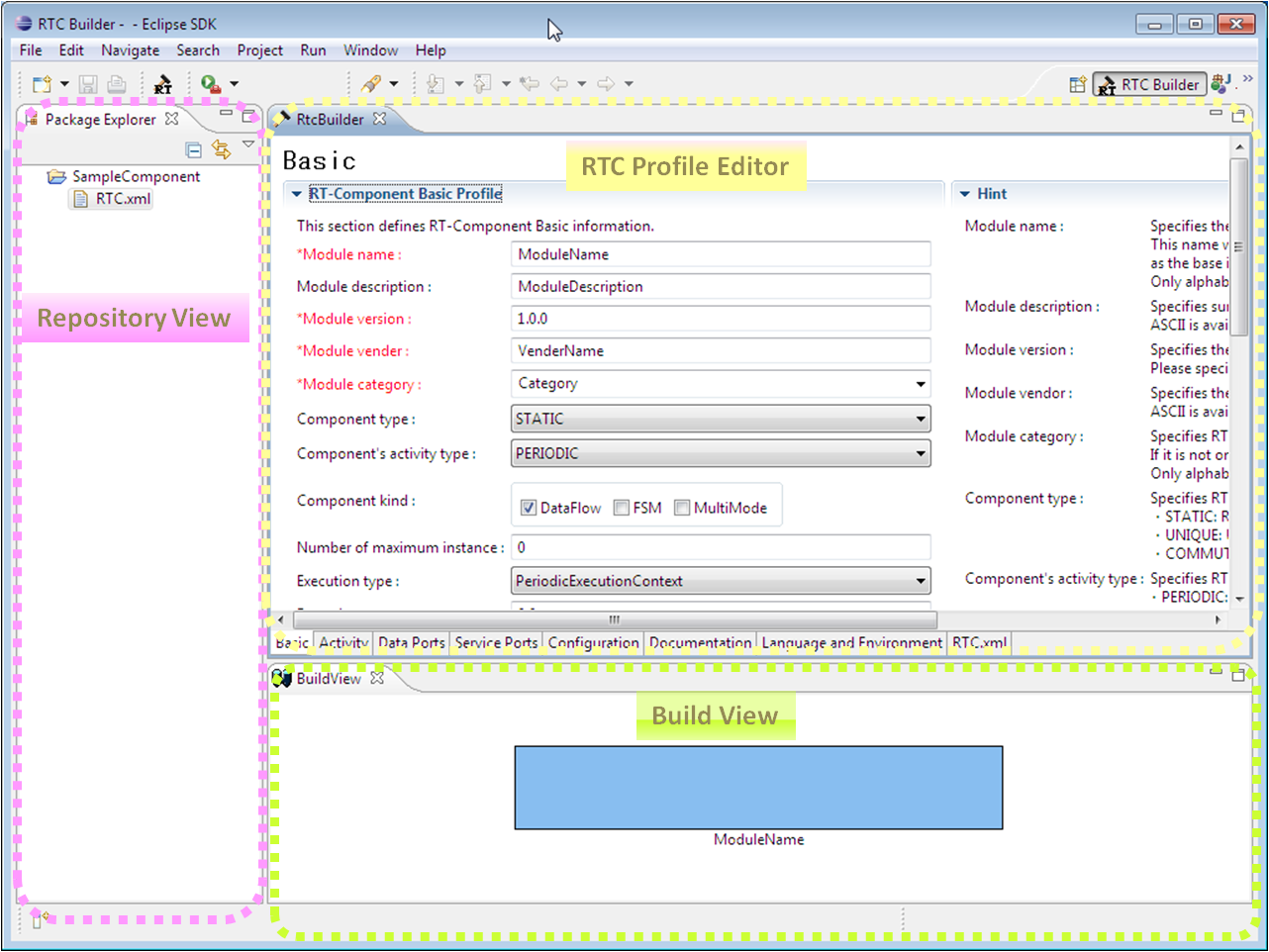
The definition of each RTC component is stored in a programming language independent xml file, and the source codes are automatically generated by the robot middleware framework using this XML file. Four source code files are created. One header and one C++ file for class definition, one C++ source file containing the main function and a makefile for building process. The developer has only to fill out the body of each skeleton member function and to insert other external classes. After building our system using these generated source we get a minimal working system, but it is hard to understand and to modify because substantial knowledge is needed about OpenRTM-aist system and the RT-specification. In the generated files the class is a subclass containing overriding methods and codes of design patterns. The knowledge of 5-10 classes are necessary for beginners. The generation process of a beginner project requires a lot of parameters at least 10, but in a complicated case can be 20-30 parameters too. C++, Java, Python programming languages Eclipse and Visual Studio are supported.
2.4.2. Component development
More than 2000 3rd party components are available for ROS that can be used freely for own robot system. Using these components the development period of the new robot system can be quick and easy. If our system is well designed i.e. the workflow of the components and the interface among them are designed precisely then the development process can be done in parallel due to available ROS tools. A message to a topic can be sent an easy way by rostopic from command line or listening to arriving messages to a specified topic. The construction of the component is not block the development of another component. Sharing a new functionality needs only a new method and variable definition and a simple function call.
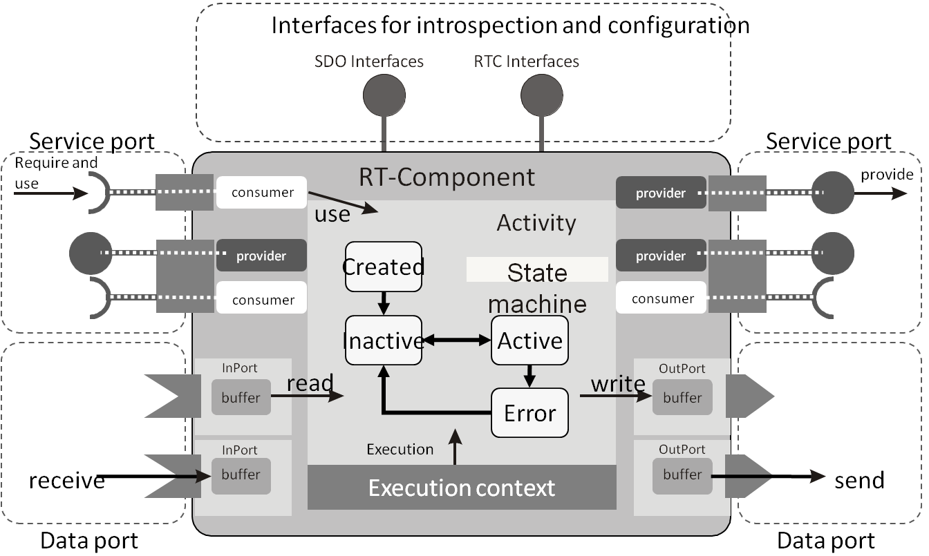
In case of OpenRTM-aist approximately 1000 components are available. Some of them can be used in Windows operating system only and the others restrict us to Linux. Unfortunately the documentation of the most components written in japan only and we have to trust the result of any language translator. The Debug and test tools are missing that helps to developer, we have to implement dummy components for this reason. In most cases the correct usage of the system services requires deep knowledge about CORBA technology that increases the full time of development. If a behaviour of any component can be used remotely we have to do more steps in the provider and consumer side also. In this case the usage of CORBA can not be omitted. The developer has to create a class containing methods of state machine and the business logic. The architecture of the component is show in the 23. ábra.
2.5. Services for end-users
The OpenRTM-aist robot framework is responsible for more services for the end-user than other ones. It supports the substitution of component, robot system creation, change of parameters of the robot, and the control of the component. Some command line tools are presented in rtc_shell package which are Python scripts. In addition, a graphical system editor is shipped as Eclipse plugin. The size of this system editor (and the Eclipse itself) is too large and the graphical capabilities are limited, but it is an effective supervisory interface of the system (the graphical interface is shown in the 24. ábra.)
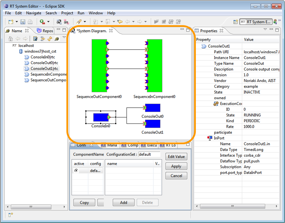
In the left side of the window the end-user can browse the online components in the middle part the actual robot system is shown. In the right side the main parameters of the component are shown. The end-user can start or stop the robot system or any component of the system at any time. If this GUI is not sufficient, than a new tool should be created. Unfortunately, the detailed documentation of OpenRTM-aist system is missing so the source code investigation is needed.
Exiguous amount of tool exist in ROS aiding the end-user. Some graphical tools are implemented in qt helping to view the log messages and draw the structure of robot system. Moreover, we should mention a promising tool that runs in a browser called Robot Web Tool. This is a Java script collection communication to the Python server application (a bridge to ROS) but additional development is necessary.
2.6. Summary for robot middleware
The OpenRTM-aist contributes more features to end-users via graphical interface, but more knowledge is needed for developer. In the case when the researcher would like to try more solutions i.e. varying the component the OpenRTM-aist is better than ROS.
It supports more programming languages and operating systems also, so it is easy to integrate it into the existing topology and easy to develop the new system. Unfortunately, the documentation is poor and some of them are exist in japan only which is not popular except in Japan. The support of more operating systems is mentioned as advantage, but it is drawbacks also, because it can lead to complicate and heterogeneous robot topology. If our robot system requires components which are found, however that components can be run only different operating system, it requires additional PC-s. The OpenRTM-ais provides more tools and features to developers, but more knowledge and experience are needed, nevertheless the documentation of the system is poor. More useful code can be found in the sample projects complementing the missing documentation, however the developer has to search it and has to try it with different parameters. An active community of OpenRTM-asit exists in Japan, nevertheless the questions and the replies are presented in Japanese language only in most cases.
The ROS is suggested in the case of autonomous system when the connection of robot parts is mandatory. In this case the graphical editor is not necessary. Because of huge number of existing components, probably one or more component exists which fulfil our requirements which are small, so the understanding and the modification are an easy task. It is easy to create a new project from the scratch (easier than OpenRTM-aist) because the creation of classes is optional we have to use existing classes and methods only. The development of the ROS core is continuous by a community, the seventh version is in progress. There are a lot of information about it and a lot of questions and answers on the web page.
2.7. References for robot middleware
|
[1] |
D. Calisi, A. Censi, L. Iocchi és D. Nardi, „OpenRDK: a modular framework for robotic software development,” in Intelligent Robots and Systems, 2008. IROS 2008. IEEE/RSJ International Conference on, 2008. |
|
[2] | |
|
[3] | |
|
[4] |
„OpenRTM-aist robot middleware official web page,” [Online]. |
|
[5] |
N. Ando, S. Kurihara, G. Biggs, T. Sakamoto, H. Nakamoto és T. Kotoku, „Software deployment infrastructure for component based rt-systems,” Journal of Robotics and Mechatronics, %1. kötet23, %1. szám3, 2011. |
|
[6] |
N. Ando, T. Suehiro és T. Kotoku, „A software platform for component based rt-system development: Openrtm-aist,” in Simulation, Modeling, and Programming for Autonomous Robots, Springer, 2008. |
|
[7] |
N. Ando, T. Suehiro, K. Kitagaki, T. Kotoku és W.-K. Yoon, „RT-middleware: distributed component middleware for RT (robot technology),” in Intelligent Robots and Systems, 2005.(IROS 2005). 2005 IEEE/RSJ International Conference on, 2005. |
|
[8] | |
|
[9] |
M. Quigley, K. Conley, B. Gerkey, J. Faust, T. Foote, J. Leibs, R. Wheeler és A. Y. Ng, „ROS: an open-source Robot Operating System,” in ICRA workshop on open source software, 2009. |
|
[10] |
K. Saito, K. Kamiyama, T. Ohmae and T. Matsuda, "A microprocessor-controlled speed regulator with instantaneous speed estimation for motor drives," IEEE Trans. Ind. Electron., vol. 35, no. 1, pp. 95-99, Feb. 1988. |
|
[11] |
A. G. Filippov, "Application of the theory of differential equations with discontinuous right-hand sides to non-linear problems in autimatic control," in 1st IFA congress, 1960, pp. 923-925. |
|
[12] |
A. G. Filippov, "Differential equations with discontinuous right-hand side," Ann. Math Soc. Transl., vol. 42, pp. 199-231, 1964. |
|
[13] |
Van, Doren and Vance J., "Loop Tuning Fundamentals," Control Engineering. Red Business Information, July 1, 2003. |
|
[14] |
C. Chan, S. Hua and Z. Hong-Yue, "Application of fully decoupled parity equation in fault detection and identification of dcmotors," IEEE Trans. Ind. Electron., vol. 53, no. 4, pp. 1277-1284, June 2006. |
|
[15] |
F. Betin, A. Sivert, A. Yazidi and G.-A. Capolino, "Determination of scaling factors for fuzzy logic control using the sliding-mode approach: Application to control of a dc machine drive," IEEE Trans. Ind. Electron., vol. 54, no. 1, pp. 296-309, Feb. 2007. |
|
[16] |
J. Moreno, M. Ortuzar and J. Dixon, "Energy-management system for a hybrid electric vehicle, using ultracapacitors and neural networks," IEEE Trans. Ind. Electron., vol. 53, no. 2, pp. 614-623, Apr. 2006. |
|
[17] |
R.-E. Precup, S. Preitl and P. Korondi, "Fuzzy controllers with maximum sensitivity for servosystems," IEEE Trans. Ind. Electron., vol. 54, no. 3, pp. 1298-1310, Apr. 2007. |
|
[18] |
V. Utkin and K. Young, "Methods for constructing discountnuous planes in multidimensional variable structure systems," Automat. Remote Control, vol. 31, no. 10, pp. 1466-1470, Oct. 1978. |
|
[19] |
K. Abidi and A. Sabanovic, "Sliding-mode control for high precision motion of a piezostage," IEEE Trans. Ind. Electron., vol. 54, no. 1, pp. 629-637, Feb. 2007. |
|
[20] |
F.-J. Lin and P.-H. Shen, "Robust fuzzy neural network slidingmode control for two-axis motion control system," IEEE Trans. Ind. Electron., vol. 53, no. 4, pp. 1209-1225, June 2006. |
|
[21] |
C.-L. Hwang, L.-J. Chang and Y.-S. Yu, "Network-based fuzzy decentralized sliding-mode control for cat-like mobile robots," IEEE Trans. Ind. Electron., vol. 54, no. 1, pp. 574-585, Feb. 2007. |
|
[22] |
M. Boussak and K. Jarray, "A high-performance sensorless indirect stator flux orientation control of industion motor drive," IEEE Trans. Ind. Electron., vol. 53, no. 1, pp. 614-623, Feb. 2006. |
|
[23] |
D. C. Biles And P. A. Binding, „On Carath_Eodory's Conditions For The Initial Value Problem,” Proceedings Of The American Mathematical Society, %1. kötet125, %1. szám5, pp. 1371{1376 S 0002-9939(97)03942-7 , 1997. |
|
[24] |
Filippov, A.G., „Application of the Theory of Differential Equations with Discontinuous Right-hand Sides to Non-linear Problems in Automatic Control,” in 1st IFAC Congr., pp. 923-925, Moscow, 1960. |
|
[25] |
Filippov, A.G., „Differential Equations with Discontinuous Right-hand Side,” Ann. Math Soc. Transl., %1. kötet42, pp. 199-231, 1964. |
|
[26] |
Harashima, F.; Ueshiba, T.; Hashimoto H., „Sliding Mode Control for Robotic Manipulators",” in 2nd Eur. Conf. On Power Electronics, Proc., pp 251-256, Grenoble, 1987. |
|
[27] |
P. Korondi, L. Nagy, G. Németh, „Control of a Three Phase UPS Inverter with Unballanced and Nonlinear Load,” in EPE'91 4th European Conference on PowerElectronics, Proceedings vol. 3. pp. 3-180-184, Firenze, 1991. |
|
[28] |
P. Korondi, H. Hashimoto, „Park Vector Based Sliding Mode Control K.D.Young, Ü. Özgüner (editors) Variable Structure System, Robust and Nonlinear Control.ISBN: 1-85233-197-6,” Springer-Verlag, %1. kötet197, %1. szám6, 1999. |
|
[29] |
P.Korondi, H.Hashimoto, „Sliding Mode Design for Motion Control,” in Studies in Applied Electromagnetics and Mechanics, ISBN 90 5199 487 7, IOS Press 2000.8, %1. kötet16, 2000. |
|
[30] |
Satoshi Suzuki, Yaodong Pan, Katsuhisa Furuta, and Shoshiro Hatakeyama, „Invariant Sliding Sector for Variable Structure Control,” Asian Journal of Control, %1. kötet7, %1. szám2, pp. 124-134, 2005. |
|
[31] |
P. Korondi, J-X. Xu, H. Hashimoto, „Sector Sliding Mode Controller for Motion Control,” in 8th Conference on Power Electronics and Motion Control Vol. 5, pp.5-254-5-259. , 1998. |
|
[32] |
Xu JX, Lee TH, Wang M, „Design of variable structure controllers with continuous switching control,” INTERNATIONAL JOURNAL OF CONTROL, %1. kötet65, %1. szám3, pp. 409-431, 1996. |
|
[33] |
Utkin, V. I., „Variable Structure Control Optimization,” Springer-Verlag, 1992. |
|
[34] |
Young, K. D.; Kokotovič, P. V.; Utkin, V. I., „A Singular Perturbation Analysis of High-Gain Feedback Systems,” IEEE Trans. on Automatic Control, %1. kötet, összesen: %2AC-22, %1. szám6, pp. 931-938, 1977. |
|
[35] |
Furuta, K., „Sliding Mode Control of a Discretee System,” System Control Letters, %1. kötet14, pp. 145-152, 1990. |
|
[36] |
Drakunov, S. V.; Utkin, V. I., „Sliding Mode in Dynamics Systems,” International Journal of Control, %1. kötet55, pp. 1029-1037, 1992. |
|
[37] |
Young, K. D., „Controller Design for Manipulator using Theory of Variable Structure Systems,” IEEE Trans. on System, Man, and Cybernetics, %1. kötet, összesen: %2Vol SMC-8, pp. 101-109, 1978. |
|
[38] |
Hashimoto H.; Maruyama, K.; Harashima, F.: ", „Microprocessor Based Robot Manipulator Control with Sliding Mode",” IEEE Trans. On Industrial Electronics, %1. kötet34, %1. szám1, pp. 11-18, 1987. |
|
[39] |
Sabanovics, A.; Izosimov, D. B., „Application of Sliding Modes to Induction Motor,” IEEE Trans. On Industrial Appl., %1. kötet17, %1. szám1, p. 4149, 1981. |
|
[40] |
Vittek, J., Dodds, S. J., „Forced Dynamics Control of Electric Drive,” EDIS – Publishing Centre of Zilina University, ISBN 80-8070-087-7, Zilina, 2003. |
|
[41] |
Utkin, V.I.; „Sabanovic, A., „Sliding modes applications in power electronics and motion control systems,” Proceedings of the IEEE International Symposium Industrial Electronics, %1. kötetVolume of tutorials, pp. TU22 - TU31, 1999. |
|
[42] |
Sabanovic, A, „Sliding modes in power electronics and motion control systems,” in The 29th Annual Conference of the IEEE Industrial Electronics Society, IECON '03, Vol. 1, Page(s):997 - 1002, 2003. |
|
[43] |
Siew-Chong Tan; Lai, Y.M.; Tse, C.K., „An Evaluation of the Practicality of Sliding Mode Controllers in DC-DC Converters and Their General Design Issues,” in 37th IEEE Power Electronics Specialists Conference, PESC '06. Page(s):1 - 7, 2006. |
|
[44] |
Slotine,J.J., „Sliding Controller Design for Non-Linear Systems,” Int. Journal of Control, %1. kötet40, %1. szám2, pp. 421-434, 1984. |
|
[45] |
Sabanovic A., N. Sabanovic. K. Jezernik, K. Wada, „Chattering Free Sliding Modes,” The Third Worksop on Variable Structure Systems and Lyaponov Design , Napoly, Italy, 1994. |
|
[46] |
Korondi, H.Hashimoto, V.Utkin , „Direct Torsion Control of Flexible Shaft based on an Observer Based Discrete-time Sliding Mode,” IEEE Trans. on Industrial Electronics, %1. szám2, pp. 291-296, 1998. |
|
[47] |
Boiko, I.; Fridman, „ L Frequency Domain Input–Output Analysis of Sliding-Mode Observers,” IEEE Transactions on Automatic Control, %1. kötet51, %1. szám11, pp. 1798-1803, 2006. |
|
[48] |
Comanescu, M.; Xu, L., „Sliding-mode MRAS speed estimators for sensorless vector control of induction Machine,” IEEE Transactions on Industrial Electronics, %1. kötet53, %1. szám1, p. 146 – 153 , 2005. |
|
[49] |
Furuta.K. , Y.Pan, „Variable structure control with sliding sector,” Automatica, %1. kötet36, pp. 211-228, 2000. |
|
[50] |
Suzuki S, Pan Y, Furuta K, „VS-control with time-varying sliding sector - Design and application to pendulum,” ASIAN JOURNAL OF CONTROL, %1. kötet6, %1. szám3, pp. 307-316, 2004. |
|
[51] |
Korondi Péter, „Tensor Product Model Transformation-based Sliding Surface Design,” Acta Polytechnica Hungarica, %1. kötet3, %1. szám4, pp. 23-36, 2006. |
|
[52] |
Vadim Utkin, Hoon Lee, „The Chattering Analysis,” EPE-PEMC Proceedings 36, 2006. |
|
[53] |
Koshkouei, A.J.; Zinober, A.S.I., „Robust frequency shaping sliding mode control” Control Theory and Applications,” IEE Proceedings, %1. kötet147, %1. szám3, p. 312 – 320, 2000. |
|
[54] |
HASHIMOTO, H., and KONNO, Y., „‘Sliding surface design in thefrequency domain’, in ‘Variable Structure and Lyapunov control’,ZINOBER, A.S.I. (Ed.) (),,” Springer-Verlag, Berlin, pp. 75-84, 1994. |
|
[55] |
Koshkouei, A.J.; Zinober, A.S.I., „Adaptive backstepping control of nonlinear systems with unmatched uncertainty,” in Proceedings of the 39th IEEE Conference on Decision and Control, pp. 4765 – 4770, 2000 . |
|
[56] |
Kaynak, O.; Erbatur, K.; Ertugnrl, M., „The fusion of computationally intelligent methodologies and sliding-mode control-A survey,” IEEE Transactions on Industrial Electronics, %1. kötet48, %1. szám1, p. 4 – 17, 2001. |
|
[57] |
Lin, F.-J.; Shen, P., „H Robust Fuzzy Neural Network Sliding-Mode Control for Two,” Axis Motion Control System IEEE Transactions on Industrial Electronics, %1. kötet53, %1. szám4, p. 1209 – 1225 , 2006. |
Chapter 3. Universal robot controller
3.1. Introduction
At the previous decades the industrial robots and NC machines becomes available for smaller companies. Industrial robots has slightly different programming mode than other Industrial machines like CNC machines and Lathes. Programming of NC machines is more standardized (G-code), while different programming languages and interfaces exist for different robots even from the same manufacturer. It is important to follow standards at production, however this standardization is absent in industrial robotics. Despite the standard G code NC machines usually do not have any appropriate port (and sometimes I/O opportunities) for high level communication in a manufacturing cell. Due to these limitations of existing NC and robot controllers, many researches were started to develop a new, open-source, flexible middleware software and hardware architecture for replacing outworn controllers [1, 13].
We are the first in the field of universal control development who are combining the following two popular existing concepts to merge their benefits: the reliable LinuxCNC and the flexible RT-Middleware technology.
The organization of the paper is as follows: Section II describes the origin of LinuxCNC software system. Section III introduces the RT-Middleware technology, Section IV presents three different concepts for hardware architecture, Section V gives an example solution with experimental results, and Section VI concludes the paper.
3.2. RS274NGC G-code standard and LinuxCNC
The US government sponsored Public Domain software systems for numeric control of milling machines were among the very first projects developed with the first digital computers in the 1950`s. In fact, the need and concepts of universal motion controllers is not a novel issue in the industry. The universality was described by modularity, portability, extensibility, and scalability requirements before two decades when the development of LinuxCNC was already started [2]. The project was originally launched by the National Institute of Standards and Technology (NIST) in 1989 [2, 3] and the software was moved under public domain in 2000, allowing external contributors to make changes and reuse the code. The characteristics of universality are still forming an actual topic as the available hardware elements are improved and the control architectures are developed. Today, LinuxCNC is a very reliable and popular open source software system that can be used under General Public License for numerical control.
3.3. Rt-middleware framework
The Japanese Ministry of Economy, Trade and Industry (METI) in collaboration with the Japan Robot Association (JARA) and National Institute of Advanced Industrial Science and Technology (AIST) started a 3 year-national project “Consolidation of Software Infrastructure for Robot Development” in 2002 [4]. An ICE Extension was proposed in [14,15]. With the intention of implementing robot systems to meet diversified users' needs, this project has pursued R&D of technologies to make up robots and their functional parts in modular structure at the software level, and to allow system designers or integrators building versatile robots or systems with relative ease by simply combining selected modular parts. The robot technology middleware have been developed as infrastructure software for implementing the proposed robot architecture, named "OpenRTM-aist" (Open Robot Technology Middleware).
To manage the rapidly growing need for sensor communication in robotic applications several suitable architectures, named middlewares, are being developed for easy system integration. Unfortunately, most of these middleware technologies are developed independently of each other and are often dedicated for specific user applications [5]. RT-Middleware is the only middleware solution that is under standardization [6] and also this solution has proved to be industry ready and used by many industrial partners: Toshiba (different system components), Honda (ASIMO humanoid robot), AIST (OpenHRP humanoid robot, etc.) and also many research institutes. The most important middleware solutions can be found in [7- 11] and a comparison can be found in [11, 12]. The main goal of the middleware system is the development of a common language and control concept for different users and tasks. The base of RT-Middleware concept is that system is build up from low-level, real-time, platform independent components (RTCs, RT-Components). These components are developed for certain machines, sensors and actuators. From these components more complex machine configurations can be made: production cells or an entire production line. The advantage of this architecture is its well-defined hierarchy, modularity, scalability and fast development ability. More details about the RT-middleware can be found in references [9].
3.4. Different architecture concepts
Following chapter describes three different experimental systems for different machines. The first is a joint controller which can be the smallest element of a manufacturing cell and controlled by an RTM server. The second is a compact 3-axis desktop CNC controller, which works as a small plug&play RT-Middleware unit. The third concept is combining the low-level flexibility (able to control different kind of systems on low level) of the LinuxCNC software system and the high-level flexibility (connectable to each other to form a production cell) of the latest RT-Middleware technology.
3.4.1. The first one is a joint controller
In case there is no hard-real-time attachment necessary between machine joints, it is possible to develop one RT-Middleware RTC hardware and software unit to drive any joint. In this concept more instances of joint component is controlled by a higher level RTC component. Main advantage of this architecture is its flexibility: new joints can be attached or joints can be reconfigured with the reuse of joint RTC hardware and software component. It has certain small delay in control which makes it not fit for example simultaneous movement of high speed CNC machine joints, but it fits to most automation applications like pick&place. An RT-Middleware based joint was developed to test the performance of this concept and get experimental results. Two pieces of this joint controller were manufactured and attached to the first two angular joints of an ADEPT 604-S type SCARA robot. Block diagram of the hardware architecture can be seen on figure IV.1. The logic was implemented in a SUZAKU-V FPGA board. Custom logic and PowerPC processor was configured to run Linux kernel and realize real-time interfaces. The board is connected to the Middleware server via Ethernet. Furthermore the developed electronics includes power amplifier for DC motors, signal conditioning and necessary power converters. It was developed to be the smallest element of a manufacturing cell.
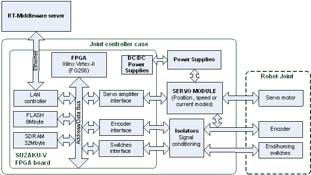
3.4.2. The second one is a simple decentralized CNC controller
At a 3 axes CNC machine the joints are usually linearly independent. In this case the joint coordinates have effects only on the X, Y and Z coordinates of the TCP. Our decentralized CNC controller can get the joint references from an external PC based G code interpreter. The mechanical design and the shape of the workspace of milling machines can be specialized for different tasks, but the control method can be the same. After the controller and the machine is connected, the position control loops of the axes run on the CNC controller (figure IV.2), and can be tuned via RS232 port from a PC. It is possible to control additional functions along output 8 relays, and 8 isolated inputs, for example coolant, tool size measurements, and other PLC functions. These I/O interfaces can be accessed along ModBus interface. With this system design and a normal PC different CNC machines can be controlled without machine specific controller development. The G code is a common machine language so the PC based RT-Middleware G code interpreter can be used universally. Our decentralized CNC controller is a universal hardware element for these machines so the cost of this concept can be reduced by the increasing number of the manufactured controllers.
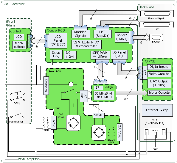
3.4.3. Linux based modular multi-axis controller
The latest version of our controllers is a complete modular solution for most motion control applications up to 9 axes. The system is based on LinuxCNC, which reliable core was developed since more than two decades, described in the introduction. And we combined this deep experience with modern hardware elements of today's semiconductor industry. This platform is an open-source software system that implements numerical control capability using general purpose computers to control any servo driven machines. It uses Linux kernel with real time extensions (RTAI or RTLinux), and can control up to 9 axes or joints of a machine using standard G-code as input. It can handle the operation of all peripheral machine elements, e.g. tool length measurement, cooling, tool-change procedure, etc. The graphical user interface can be customized for specific kinds of usage e.g. touch screen or interactive development, see figure IV.3. Programming features include most needs of NC usage. It is possible to implement inverse kinematics, hence the software system is capable to control non-Cartesian robots as well. The hardware architecture of the generic system layout can be seen on figure IV.4. The PC installed with LinuxCNC is hosting a PCI card, which is based on a PCI bridge ASIC and an FPGA.
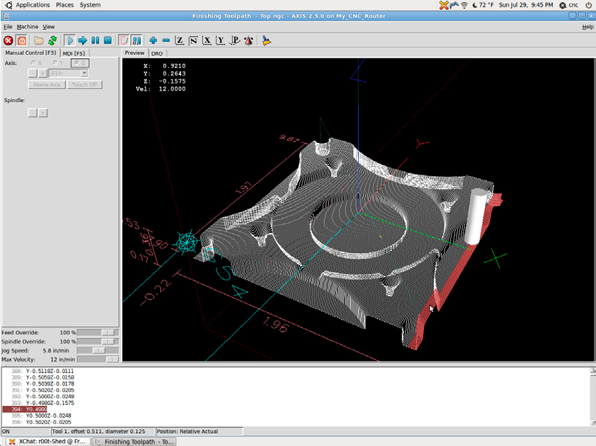
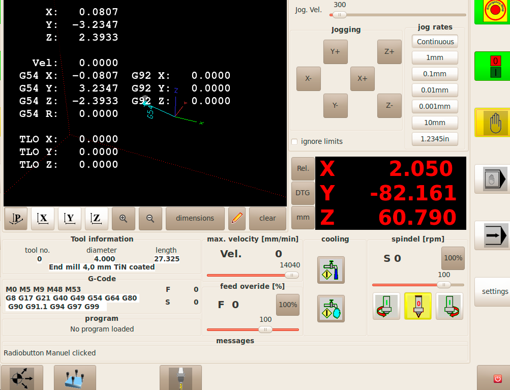
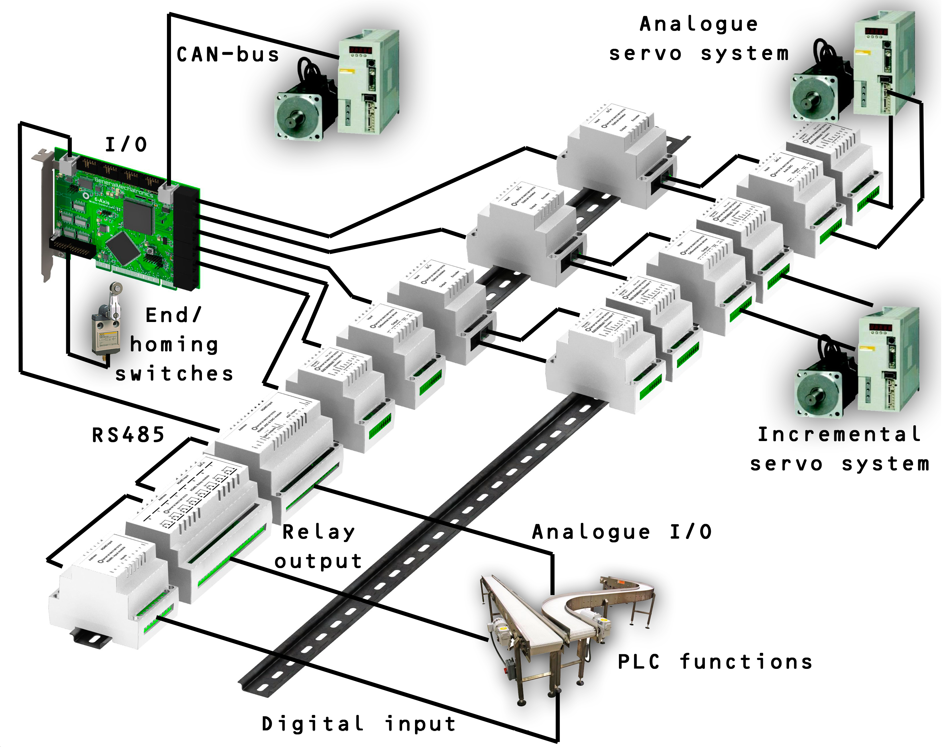
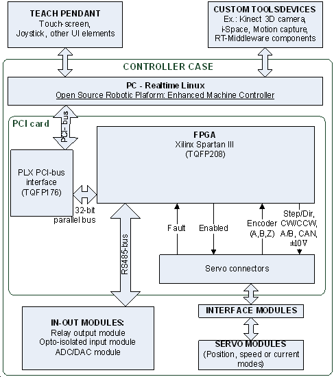
(b)
As the LinuxCNC has a simple ladder diagram editor and handles standard PLC functions, the hardware architecture is extended with a RS485 bus for I/O extension modules. The bus is handled by a separate 8-bit RISC microcontroller on the PCI card, which communicates via SPI with the FPGA. Currently digital input, relay output, ADC/DAC, and teach pendant modules are exist. These modules can be connected in chain with a termination resistor at the end of the bus, see figure IV.5./a. Each module has a unique, four bit long address on the bus, hence up to 16 modules can be chained to one PCI card.
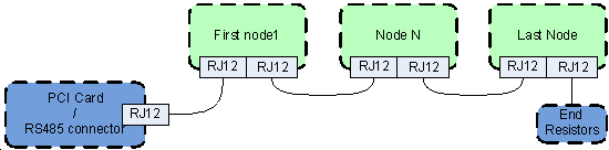

Basically, the modules have a bus powered and a field or application powered side with an optical isolation between them, see figure IV.5./b. But for example an optical isolated input module has only field power side as the inputs from the field are only simple opto-coupler inputs. Each node connected to the bus is recognized by the PCI card automatically. During startup the driver exports pins and parameters of all available modules automatically. All the I/O-s of these modules can be routed to a function in the hardware abstraction layer (HAL) of LinuxCNC, and can be controlled by a custom logic implemented with the ladder editor.
The specialty of the system is in the servo connection interface. A novel modular concept is introduced for connecting different types of servo controllers including the old analogue systems, the incremental systems, and modern CAN based servo modules. Four different small and simple axis-interface modules were developed, and combining them in many different ways makes the possibility of interfacing with a servo controller. These types are optical isolator, DAC module, differential line driver, and a breakout for simple terminal connection. Figure IV.6. shows only two different servo examples from the possible 8: a analogue, and an incremental with differential outputs and encoder feedback.
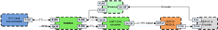
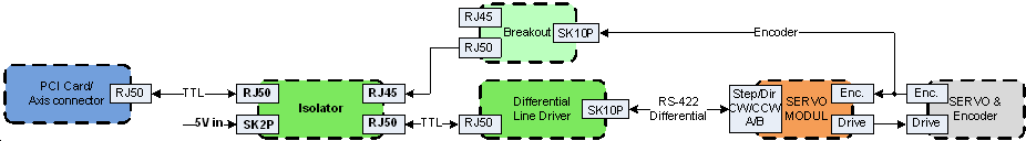
3.5. Example solution
This chapter presents an application to multi-axis simultaneous control. LinuxCNC was connected to a SCARA type robot. The theoretical background of the implemented control algorithm is described in point A). The modular hardware structure resulted a flexible system which can be connected to any similar machines without long time demanding hardware development (described in point B).
3.5.1. Kinematics of the experimental non-Cartesian system
Three different universal architectures were introduced from which two were connected to a SCARA type robot. This chapter describes the implemented SCARA kinematics (Fig. V.1.) which is followed by hardware and driver-level software description of an experimental systems.
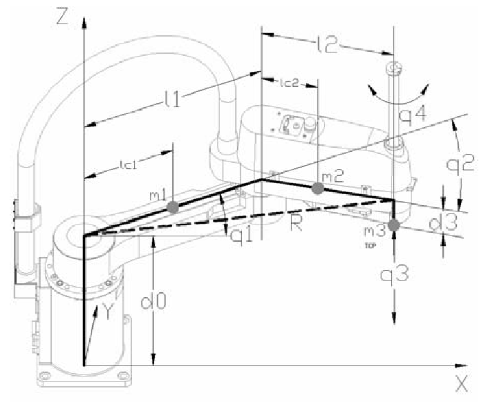
The Cartesian coordinates of TCP can be expressed as equation (5.1), (5.2), (5.3).
|
|
(5.1) |
|
|
(5.2) |
|
|
(5.3) |
Forward kinematics can be expressed deriving equations (5.1), (5.2) as (5.4),(5.5).
|
|
(5.4) |

|
|
(5.5) |

The connection between the Cartesian velocities and joint velocities can be represented as equation (5.6).
|
|
(5.6) |

Where

Where  is a Jacobean matrix as equation (5.7)
|
|
(5.7) |
3.5.2. Application example
At a manufacturing line an assembler or palletizing cell is usually indispensable. The most common palletizing type robot is the SCARA. The LinuxCNC has a kinematic module, which software part is open source as well. We designed the kinematic module for a SEIKO D-TRAN TT 4000SC SCARA robot. The original controller was broken and obsolete, but the mechanics of the machine worked perfectly. Our controller has a modular built up, so the main parts of the system are separated in three shelves. The first one is universal for most kind of machines which is the PC and the PCI card. (Fig.V.2.a) The machine specific signals (end- and homing- switches), the RS485 bus, and the CAN references are also connected to this part of the controller.
The second shelf contains the modular components, which is chosen for the specific machine. In this case these are the DC power amplifiers and the RS485 modules. (Fig.V.2.b) (These can be digital and analogue I/O-s.) The power amplifiers are connected to the DC bus, to DC logic power, to CAN references and to the encoders. The motor parameters, the encoder parameters and control loops at the power amplifiers can be tuned and measured via USB.
The third shelf contains the power electronics. (Fig.V.2.c) These elements are mainly saved from the original controller. It has an E-Stop circuit, fuses, DC powers, brake resistors and thermal protection. With this concept we could save and modernize the original robot mechanics (and some of the power electronics). The machine can be integrated into a modern and flexible manufacturing line as a palletizing cell. According to the modular built up of the controller we could use the SCARA robot again without any long time demanding electronic and software development. As a part of the system we also developed a teach pendant with touch screen and joysticks for the X,Y,Z and rotZ jogging. The controller has standard Ethernet, USB, etc. interfaces. With the LinuxCNC RT-Middleware component the robot can be connected and integrated into a high level manufacturing control system.
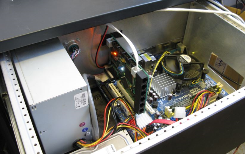
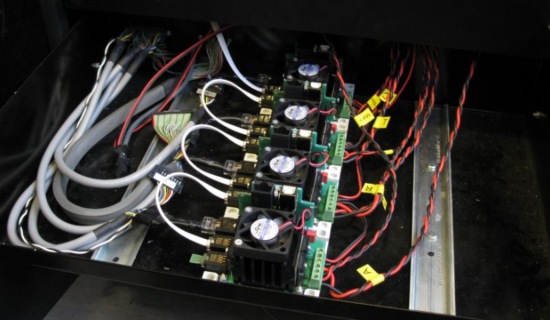
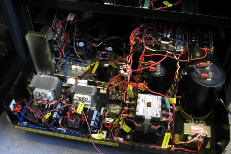
3.6. Conclusion for the universar robot controller
The LinuxCNC & RT-Middleware based modular control system was implemented with success for more machines now: Two 3-axes desktop CNC, a 3-axes dental CNC, a 5-axes with tool-change and tool-length measurement, and at least two SCARA robots. All of these machines can be connected along the RTM interface of the LinuxCNC and can work together in real-time applications. The improvement of the modules and all other hardware elements was in progress with every system integration. The first controller was running since more than one year with negligible maintenance now, showing that the system is reliable too. The application was started by external international system integrators in Europe this year.
3.7. References for the Universal robot controller
Bence Kovács, Géza Szayer, Ferenc Tajti, Solvang Bjorn, Péter Korondi, Design of a universal robot controller Robi, International Engineering Symposium at Bánki (IESB 2011). Budapest, Hungary, pp. 1-13, 2011.11.15.
Proctor, F. M., and Michaloski, J., "Enhanced Machine Controller Architecture Overview," NIST Internal Report 5331, December 1993. Available online at ftp://129.6.13.104/pub/NISTIR_5331.pdf
Albus, J.S., Lumia, R., “The Enhanced Machine Controller (EMC): An Open Architecture Controller for Machine Tools,” Journal of Manufacturing Review, Vol. 7, No. 3, pp. 278–280, September 1994.
Bence Kovács, Géza Szayer, Ferenc Tajti, Péter Korondi, István Nagy: "Robot with dog type behavior”, 17th Int. Conference on Electrical Drives and Power Electronics The High Tatras, Slovakia 28–30 September, 2011
Kotoku, Tetsuo: "Robot Middleware and its Standardization in OMG" in International Conference on Intelligent Robots and Systems (IROS'06) Workshop on Robotic Standardization, Beijing, China, 11-13 Oct. 2006
J.U. Cho, Q.N. Le and J.W. Jeon, An FPGA-Based Multiple-Axis Motion Control Chip, IEEE Trans. Ind. Electron., Vol. 56, No. 3, pp. 856-870, Mar. 2009.
Ozaki Fumio, Oaki Junji, Hashimoto Hideaki, Sato Hirokazu, "Open Robot Controller Architecture (ORCA)" in Journal: Nippon Kikai Gakkai Robotikusu, Mekatoronikusu Koenkai Koen Ronbunshu, Vol. 2, 2003.
M. Mizukawa, H. Matsuka, T. Koyama, T. Inukai, A. Noda, H. Tezuka, Y. Noguchi, N. Otera, "ORiN: open robot interface for the network - the standard and unified network interface for industrial robot applications" in Proceedings of the 41st SICE Annual Conference (SICE 2002), Tokyo, Japan, Vol. 2, pp. 925- 928, Aug. 2002.
N. Ando, T. Suehiro, K. Kitagaki, T. Kotoku, Yoon Woo-Keun, “RT-middleware: distributed component middleware for RT (robot technology)” in Proceedings of 2005 IEEE/RSJ International Conference on Intelligent Robots and Systems (IROS 2005), pp. 3933- 3938, ISBN: 0-7803-8912-3, 2-6 Aug. 2005.
G. Veiga, J. N. Pires,K. Nilsson “On the use of SOA platforms for industrial robotic cells” in Proceedings of Intelligent Manufacturing Systems (IMS2007), Spain, 2007.
J.-C. Baillie, “URBI: towards a universal robotic low-level programming language” in Proc. of IEEE/RSJ International Conference on Intelligent Robots and Systems (IROS 2005), pp. 820- 825, ISBN: 0-7803-8912-3, 2-6 Aug. 2005.
B. Solvang, G. Sziebig, and P. Korondi, “Multilevel control of flexible manufacturing systems,” in Proc. IEEE Conference on Human System Interactions (HSI’08), pp. 785– 790, 2008.
Solvang Bjørn, Refshal Lars Kristian, Sziebig Gábor “STEP-NC Based Industrial Robot CAM System.” In: 9th IFAC Symposium on Robot Control (SYROCO2009). Gifu, Japán, 2009.09.09-2009.09.12. (IFAC) Gifu: IFAC by Pergamon Press, pp. 361-366.
Zoltán Krizsán, “ICE Extension of RT-Middleware Framework”, in Proceedings of 10th International Symposium of Hungarian Researchers on Computational Intelligence and Informatics, pp 513-521, 2009.
Zoltán Krizsán, Szilveszter Kovács: Structural Improvements of the OpenRTM-aist Robot Middleware, Applied Computational Intelligence in Engineering and Information Technology Topics in Intelligent Engineering and Informatics, Eds: R.E. Precup, S. Kovács, S. Preitl and E.M. Petriu, 2012, Volume 1, pp. 287-300, ISBN: 978-3-642-28304-8
Chapter 4. Internet-based Telemanipulation
- 4.1. Abstract
- 4.2. Introduction
- 4.3. General approach of telemanipulation
- 4.4. Master devices as haptic interfaces
- 4.5. Animation of the operator’s hand wearing the sensor glove
- 4.6. Overview of control modes
- 4.6.1. Basic Architectures
- 4.6.2. Nonlinear scaling (Virtual coupling impedance)
- 4.6.3. Time delay compensation of internet based telemanipulation
- 4.6.4. Friction compensation for master devices
- 4.7. A complete application example: A handshake via Internet
- 4.8. Conclusions for telemanipulation
- 4.9. References for telemanipulation
4.1. Abstract
The Internet is a very fast evolving new technology, allowing people to electronically connect places that are thousands of miles apart. By combining network technologies with the capabilities of mobile robots, Internet users can discover and physically interact with places far away from them, creating opportunities in resources sharing, remote experimentation and long-distance learning. This paper provides an assessment of the state of art of Internet based control and presents a general approach to internet based telemanipulation. The concept is based on layers. This paper proposes these layers as well as their functions. One of the most important problems of a closed-loop internet-based telemanipulation application is the transmission time delay, which can destabilize the system. Furthermore, when using a computer network for sending data, time delay is not even constant. In this paper the Internet transmission time delay is discussed, various remote control modes for robotic systems are surveyed and an internet-based tele-handshaking as an applications is discussed in details. The task is to realize a handshake between two people at two different corner of the world via Internet.
4.2. Introduction
4.2.1. Brief History of Telemanipulation
In about 1945 the first modern master-slave system teleoperator was developed by Goertz at Argonne National Laboratory (ANL) [1]. This system, which was a mechanical pantograph mechanic system, allowed a human operator to manipulate radioactive materials in a “hot cell” from outside. By using a master handle, the human operator could move the slave tong located inside the hot cell and receive force reflection. Soon (in 1954) electrical servomechanisms replaced the direct mechanical master-slave system and able linkages [2]. Closed circuit television was introduced so that the operator could stay at an arbitrary distant place. In addition, the contact force between the slave and its environment was returned to the master arm. In 1964, Mosher developed an impressive work, which was a handy-man containing electrohydraulic arms. Each arm had ten DOF in each arm. The problem of remote control of robotic systems has been the subject of much research in recent years. Remote control of robotic systems has been applied in manufacturing, underwater manipulation, storage tank inspection, nuclear power plant maintenance, space exploration, etc. See en excellent review of relevant historical development in telemanipulation (telerobotics) in [1].
4.2.2. What is Telemanipulation
Telemanipulation is a process where the operator has some task done at the remote hazardous or inaccessible environment as space, underwater, nuclear plants, where he/she cannot physically be. A teleoperator system extends the operator’s capability to be able to work at the Remote Workplace. This extension is achieved by a master-slave system. Telemanipulation is divided into two strongly coupled processes. One process is the interaction between the operator and the master device, the other is the interaction between the slave device and the remote environment contact. The master device represents the distant environment at the operator site, and the slave device represents the operator at the remote site. When humans use this device only to move objects and the reaction force from the distant environment has no significant effect on the performance, than measurement of the operator’s position and visual feedback may be enough. However, if such tasks are to be performed when the reaction of the environment is important and the salve device can do damage in the remote environment for example when screwing a bolt or assembling something, then a force feedback is needed to improve efficiency. Force feedback increases the feeling of being there. The information flow between the operator and remote site can be seen in 4-1. ábra (adapted from [3]), where only three types of information are feedback: visual, audio and sense of touch. A human being receives five types of sensing from his/her surrounding environment but only some of these senses are used during telemanipulation.
![Information streams of the Telemanipulation (adapted from [3])](images/image_29.png)
The structure of this paper is as follows. The next section overviews the general approach of telemanipulation. It introduces three main layers of a telemanipulation system. Section 3 summarizes the basic type of master devices. Section 4 provides a short introduction into control modes used for telemanipulation. Section 5 is an application example of a handshaking via Internet.
4.3. General approach of telemanipulation
4.3.1. Basic definitions
4-2. ábra shows the general concept of telemanipulation. The “world” is divided into two sets: the Master Site and the Slave Site. The master-slave system is realized as two information channels: Action and Reaction channel. The Action channel transfers the information from the operator to the Remote Workplace. The Reaction channel transfers the information to the opposite direction: from the Remote Workplace to the Operator. In the early days of telemanipulation, the human operator’s hands and the remote environment were mechanically coupled. The information was transferred mechanically, that limited the type of the tasks, which they could perform. Nowadays, the information is transferred electrically, that opened a new dimension at the slave side. A Human-Robot System may be considered as a type of telemanipulation, where a human and a robot work simultaneously together to achieve a task. For example, in the case of remotely deactivating of a bomb, the robot must reach the bomb and than the timer must be disassembled with the help of a pair of slave manipulators. In this example the navigation and manipulation tasks may be separated. When a group of mobile robots move a large object cooperatively the operator must control the overall action. In general, the Slave Device can be a Multi Robot System as well, where more than one robot are working together to achieve a task. Computer Networked Control enables systems to be distributed. The concept of an operator and robot can be replaced with some combination of multiple operators, multiple robots, and maybe even multiple assistant agents that work together in a cooperative environment [4]. The Human-Robot type of telemanipulation can be classified into
Single master-- single slave
Multi-master-- single slave
Single master -- multi-slave
Multi-master-- multi-slave
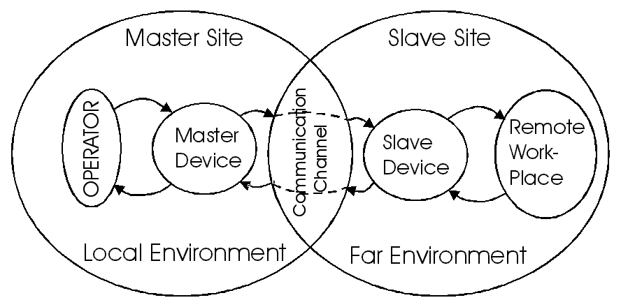
We can conclude that the meaning of telemanipulation has extended, and new terminologies have appeared. Some of them collected here.
Teleoperator is the machine itself, which can perform the task in a distant place. Using a general sense of teleoperator, Telerobot is a subclass of it. Originally, telemanipulation means the action in which a slave manipulator tracks the motion of master manipulator. In this case the salve and master manipulator have the same structure. The extension of this concept means a manipulation in the remote environment with a slave device controlled by a master device moved by a human operator. Using this extended meaning, the structure of master and slave device can be different but the whole manipulation process is controlled by the human operator, i.e. the slave side has no own intelligence. The next step is the distribution of intelligence. The slave device may learn the behavior of a human operator and may follow the learned behavior during the period when the command is delayed because of the latency caused by Internet communication [5]. Some authors use the word of teleoperation for the extended meaning of telemanipulaton, some authors use “telemanipulation” and “teleoperation” in the same sense.
A human operator needs the illusion of direct contact with the remote environment to perform fine task such as tele-surgery or remote assembling (disassembling) fine mechanism (timer bomb). A human operator receives five types of sensing (sight, hearing, touch, smell, taste) but the combinations of the first three are used during a manipulation. The psychological feeling of “being there” in an environment based on a technologically founded immersion environment called as Telepresence [6,7], which is should provide the ideal sensation, i.e. we get the necessary information fed back from the slave to the master side in a natural way to have the feeling of being physically at the distant location. Telepresence systems are a subclass of teleoperators. The technology of audio-visual feedback is well developed and available nowadays. The main challenge is the haptic feedback, which is necessary to feel the physical contact with the environment. It is an extension of force feedback. A human operator has different types of receptors for sensing different types of contact forces. Tactile (cutaneous) feedback is sensed by mechanoreceptive nerve endings in the glabrous skin (especially in the finger tips). Its bandwidth is about 50-350 Hz [8]. It provides information of small-scale details, for examples that of the type of surface. The force (kinesthetic) feedback has lower bandwidth (up to 10 Hz) sensed by receptors on the muscle tendon and in skeletal system. It provides information related to body posture. Force feedback not only increases efficiency, but it helps to filter the smaller imprecision of the operator.
4.3.2. Ideal Telepresence
In a typical telepresence, information about task at the remote site is required to help a human operator to feel as if he/she physically is present at the remote place. Accordingly a teleoperator must provide complete transparency, which means the positions, velocities, and forces of the master and slave device are equal. An example of simple remote device is a remote plier used to handle objects in a nuclear plant [5]. If this plier is stiff and easy to move, the operator simply performs the task. Images of the ideal connection between the master and slave for revolute motion and linear motion are shown in REF _Ref364272027 \h (a) and (b). If the operator rotates (move) the master stick by qm (xm) the motion of the slave stick must be the same (qm= qs or xm= xs) and the operator must sense the reaction force of the environment (Fo=- Fe), in ideal case. From this example, the aimed dynamic behavior of the teleoperator is therefore close to a rigid rod which mechanical properties are minimal inertia and maximal stiffness. The connection of the master and slave arms should have 0 mass with stiffness.
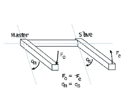
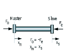
However our work deals with a teleoperator with time delay whose master and slave are assumed to be physically equivalent. The ideal responses for the Telemanipulation with time delay are definite and as follows.
The teleoperator must remain stable.
The force that the human operator applies to the master arm is equal to the force reflected from the environment in the steady state. This can help operators to realize force sensation.
The master position is equal to the slave position in the steady state.
4.3.3. Layer Definitions
The Master Site and the Slave Site are partitioned to three main layers (see in 4-4. ábra). The layers can communicate vertically with the local layers as well as horizontally with the remote layers via the Internet. The Sensor Layer contains the necessary sensors to observe the Remote Environment, and the Remote Workplace. In general, these sensors are non-contact sensors. The Manipulator Layer makes the effective work in the Remote Workplace. This layer involves the Slave Device typically. This layer may contain contact sensors. The Transporter Layer includes a Transporter (mobile unit), which can carry the slave device. The Monitor Layer at the Master Site shows the processed data of the Sensor Layer. These monitors are usually non-contact displays or indicators. The Manipulator Layer has a real contact with the Operator. This layer involves the Master Device typically. This layer, included with the Master Device, may contain contact sensors, and contact actuators. The contact actuators relay the sensed data of the contact sensors of the Manipulator Layer. The Transporter Control Layer controls the Transporter at the Slave Site. This layer may contain services that can help to the navigation of the Transporter Layer at the Slave Site.
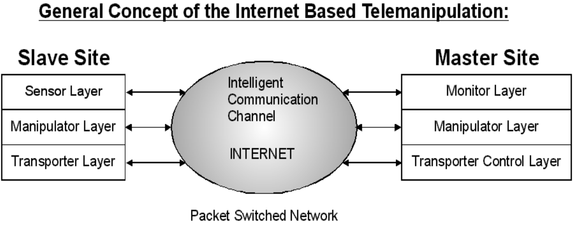
4.3.4. Sensor layer
The configuration of the Sensor Layer can be seen in 4-5. ábra. The non-contact sensors on the Slave Site are observing the Far Environment. The Intelligent Sensed Data Computing System at the Slave Site is a preprocessor for the sensed data. The purpose of this device is filtering, correction and compression. The audio and video compression formats are widely used on the Internet, to decrease the necessary bandwidth. The Computing System may contain a pattern recognition module to improve the efficiency and intelligence of the Slave Site. The purpose of the Intelligent Sensed Data Computing System at the Master Side is data decompression and recovery of lost data.
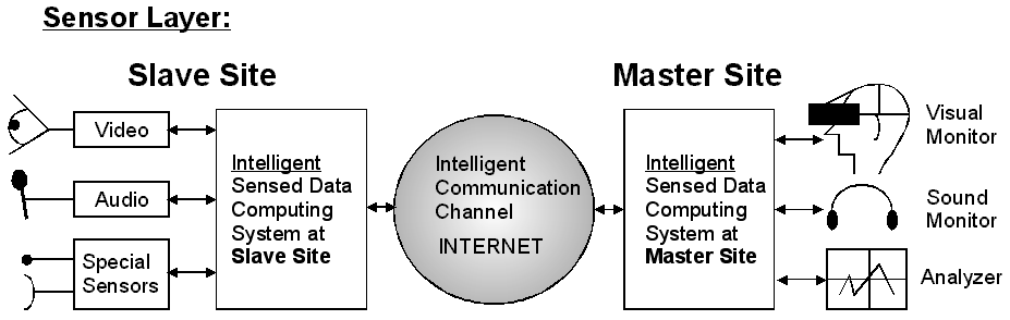
4.3.5. Manipulator layer
There is another approach for the telemanipulation. The process of the telemanipulation can be partitioned into two coupled sub-processes. One sub-process is running in the Local Environment: Local Process. The other sub-process is running in the Remote Environment: Remote Process. The Local Process is the information circulation between the Operator and the Master Device. The Distant Process is the information circulation between the Slave Device and the Remote Environment. If telemanipulation is ideal, the two processes are the same. In case of ideal telemanipulation, the Master Device represents the Remote Workplace in the Local Environment and the Slave Device represents the Operator in the Far Environment. The Communication Channel is the coupler between the two sub-processes. The main task of the Communication Channel is to ensure total transparency in case of ideal telemanipulation.
The configuration of the Manipulator Layer can be seen on 4-6. ábra. Typically, this layer includes the Slave and the Master device, as it is mentioned above. The main purpose of this layer is the position control and the force-feedback. The force-feedback is an information flow between the layers and between the Master and Slave Site. The force- feedback is a typical action-reaction process. The exact realization of the force-feedback depends on the specific approach. The configuration of the Master Device is not equal to the configuration of the Slave Device in a general case. The main purpose of the Intelligent Path Planning is to couple the master and the slave in position and force.
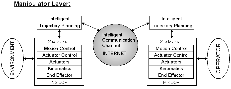
4.3.6. Transporter layer
The configuration of the Transporter Layer can be seen in 4-7. ábra. The configuration of the Slave Site of Transporter Layer is very similar to one side of the Manipulator layer. The Transporter Layer has connection with the Far Environment. The Transporter Layer carries the Slave Device and the necessary sensors.
The Task Oriented Path Planning System controls the transporter on the Slave Side. This device may use advanced services for navigation such as Global Positioning System (GPS), Geographic Information System (GIS) and Intelligent Transport System (ITS).
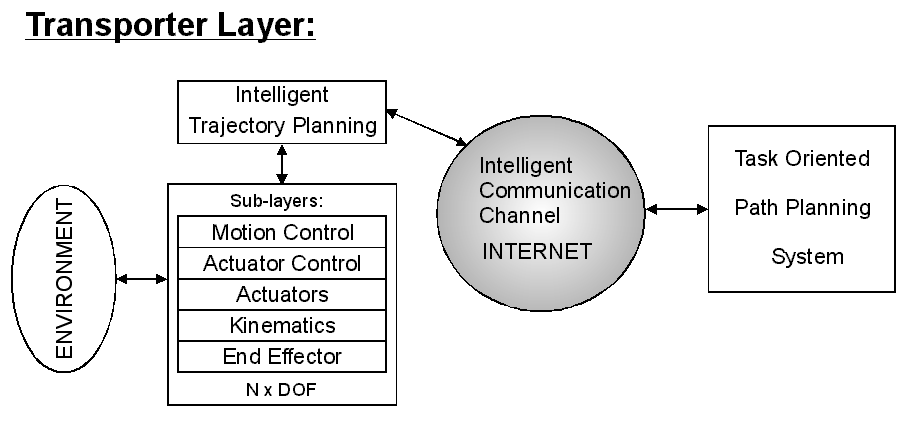
4.3.7. Special types of telemanipulation
Telemanipulation in virtual reality is beneficial when an operator is learning to perform dangerous or difficult tasks such as working with radioactive materials or disassembling explosives; or driving an airplane, helicopter or submarine in a real time simulator. In addition “Flight and other vehicles simulators” are very popular in the field of entertainment. It can be a very attractive target in both main fields professional and commercial. Telemanipulation in a virtual reality application is shown on 4-8. ábra. The operator wears a head-mounted device that provides visual feedback and an arm and glove type master device giving tactical sensation. The operator can see the visual objects and can touch and move them [10].
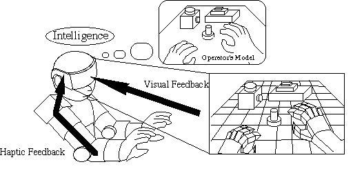
Micro- and nano-technology opened a relatively new, emerging dimension in the field of telemanipulation. Going from macro to micro/nano world, the main phenomenon is the reduction of the size of objects where the effect of length change is defined as scaling. It is obvious that Force and position must be scaled (see in 4-9. ábra). There is another problem called as bandwidth effect, that means bandwidths of the master device including human operator’s reaction and slave device including nano/micro environment are different. The micro/nano actuator has a smaller time constant than the macro force feedback device. So an impedance scaling is necessary to avoid instabilities and unreliable force feeling. It can be considered as a kind of time scaling. In another words, the micro/nano phenomena might be to fast for a human sensation and it must be slowed down by virtual coupling impedance. [11]
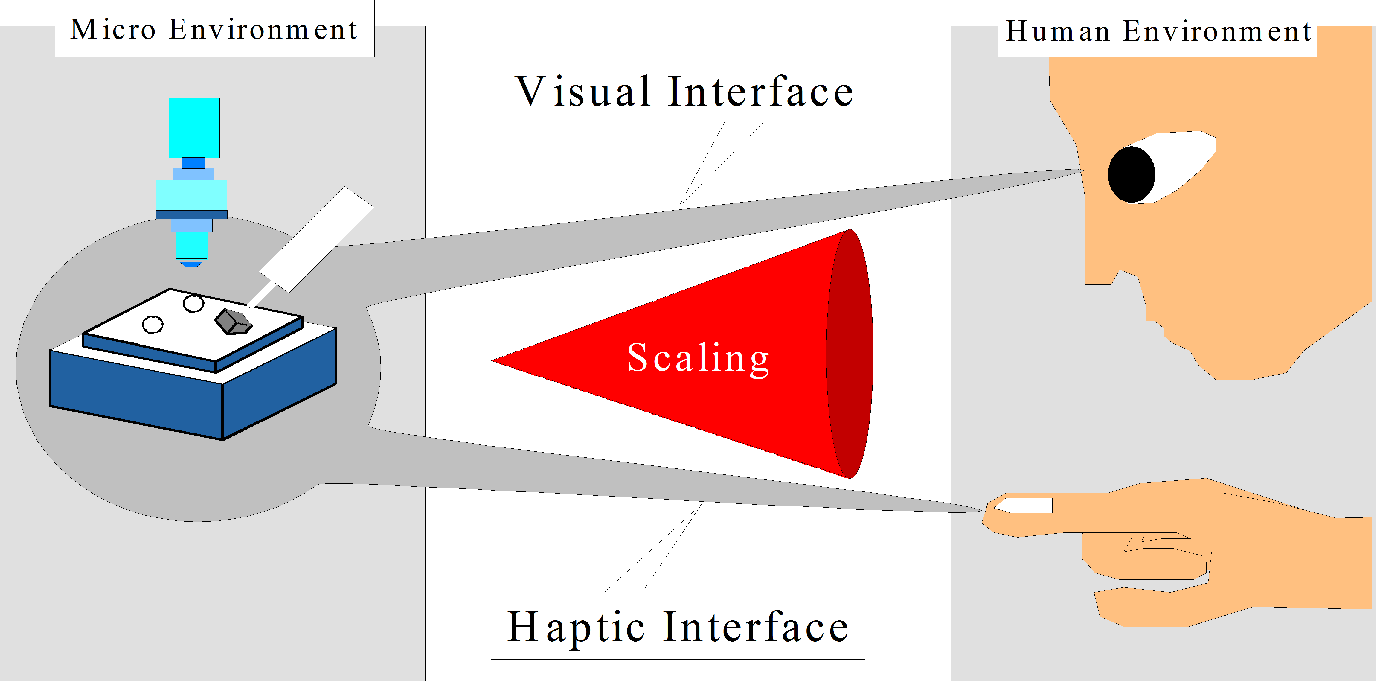
4.4. Master devices as haptic interfaces
Human operators perform their tasks mostly by hand and the master device must fit the operator’s hand. In the field of telemanipulation, many haptic devices have been developed. The applications of the haptic devices cover various fields, such as medical application, working in nuclear power plants and entertainment. In this section four important master device concepts are presented.
4.4.1. Joystick with force feedback
It was developed in the early stage of telemanipulation. Nowadays several commercial joysticks with force feedback are available. This device is optimal for low quality telemanipulation application. This device is optimal for "pick and place" operation. Joystick with force feedback is very popular in recent video game systems. Another important application area is the real time simulators of vehicles, such as airplanes, helicopters, and submarines. The main problem with these devices is the dynamics change "on the fly". An additional device is needed for balancing the dynamics of the joystick. This feature is necessary in application where different precision operations are required. Another disadvantage of the device is the two controlled degrees of freedom.
4.4.2. The point type master device
It similar to a six DOF manipulator. The operator can point at the remote site. The Phantom [12] is a point type device (see 4-10. ábra) using direct drive and is noted for its high resolution. However it can cover only fingertips. The operator can control a tip type slave device with this device. Tip type slave systems are widely used in surface manipulation applications, such as telemanipulation in the nano space [11].
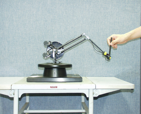
4.4.3. The arm type master devices
It covers the human arm from shoulder to wrist (see in in 4-11. ábra). It has 6 degrees of freedom. The arm type haptic device is useful in applications where the operator uses his arm to do some task in the remote environment, for example some mining workplace. In several applications the arm type master device is a subsystem of a complex master device.
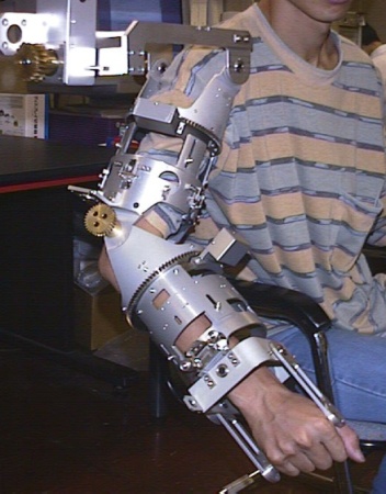
4.4.4. The glove type master device
It allows the most complex and dexterous manipulation [13]. The human hand is the most widely used tool. The final goal is to make such a device that the operator can feel as if the function of whole his hand were expanded. Several types of manipulation cannot be performed without force feedback. A 20 DOF sensor glove type device with force feedback (see in 4-12. ábra) is discussed in the next section.
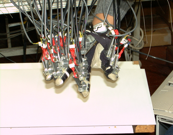
4.4.4.1. Mechanical structure
The wrist location is measured by an inductive sensor. The sensor glove is equipped with force feedback capability to each joint of the operator fingers, so the operator can feel the remote environment as he/she is there. The mechanical structure of a finger is shown in 4-13. ábra. The device is designed with consideration to the space for sensors and actuators. The device is attached to a human hand by bands. A fixed base for all movements of the glove is constructed on a metallic plate fixed on the back of human palm. Five yawing drive units are fixed in the plate. Three pitching drive components are placed on the yawing drive units.
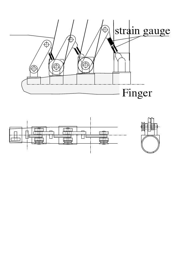
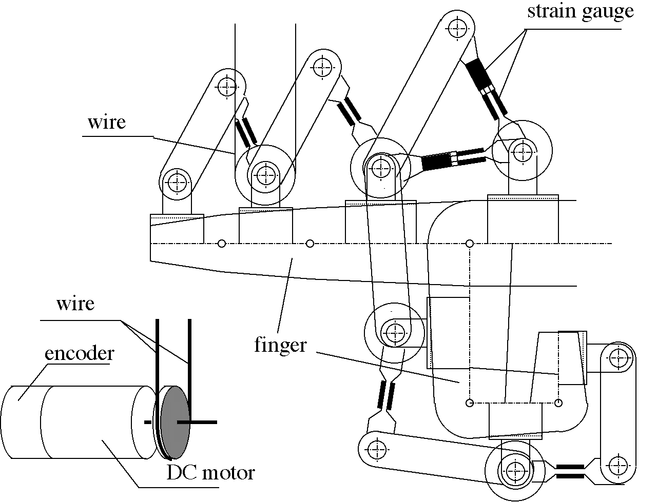
4-15. ábra shows the structure of one D.O.F. of the device. The torques of the finger joints are measured by strain gauges. Rotary encoders in the motors are used to measure the angles of the joints. Ideally, the motors move the joints directly, however, there was no motor available which was small and light enough to be attached on the hand. The pulleys and wires in tubes are used to transmit forces to the motors. Single motors can control all the 20 joints of a human hand independently. One joint of the finger corresponds to 2 links of the device. The main problem is the friction. Because of this additional force, the operator cannot feel, which force is emerged in remote environment. The friction compensation is discussed in Session IV.
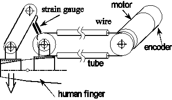
4.4.5. Micromanipulation Systems
In this section, the tele-micromanipulation system is introduced (see 4-16. ábra). In micromanipulation, visual information of microenvironment is usually fed back by microscope. It is difficult to manipulate micro object using only 2D visual information that is why a 3D animation of slave device (see left part of 4-16. ábra) helps the operator. In this system, the master input device used by the human operator is called as haptic interface, which is a 6 DOF joystick type master device (see in 4-17. ábra). The slave manipulators used directly to perform manipulation tasks are shown in 4-18. ábra. The slave manipulator and master device systems are connected using Ethernet and they are used to perform teleoperation through the network.
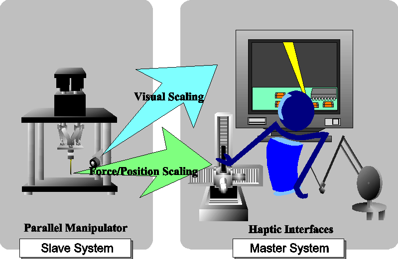
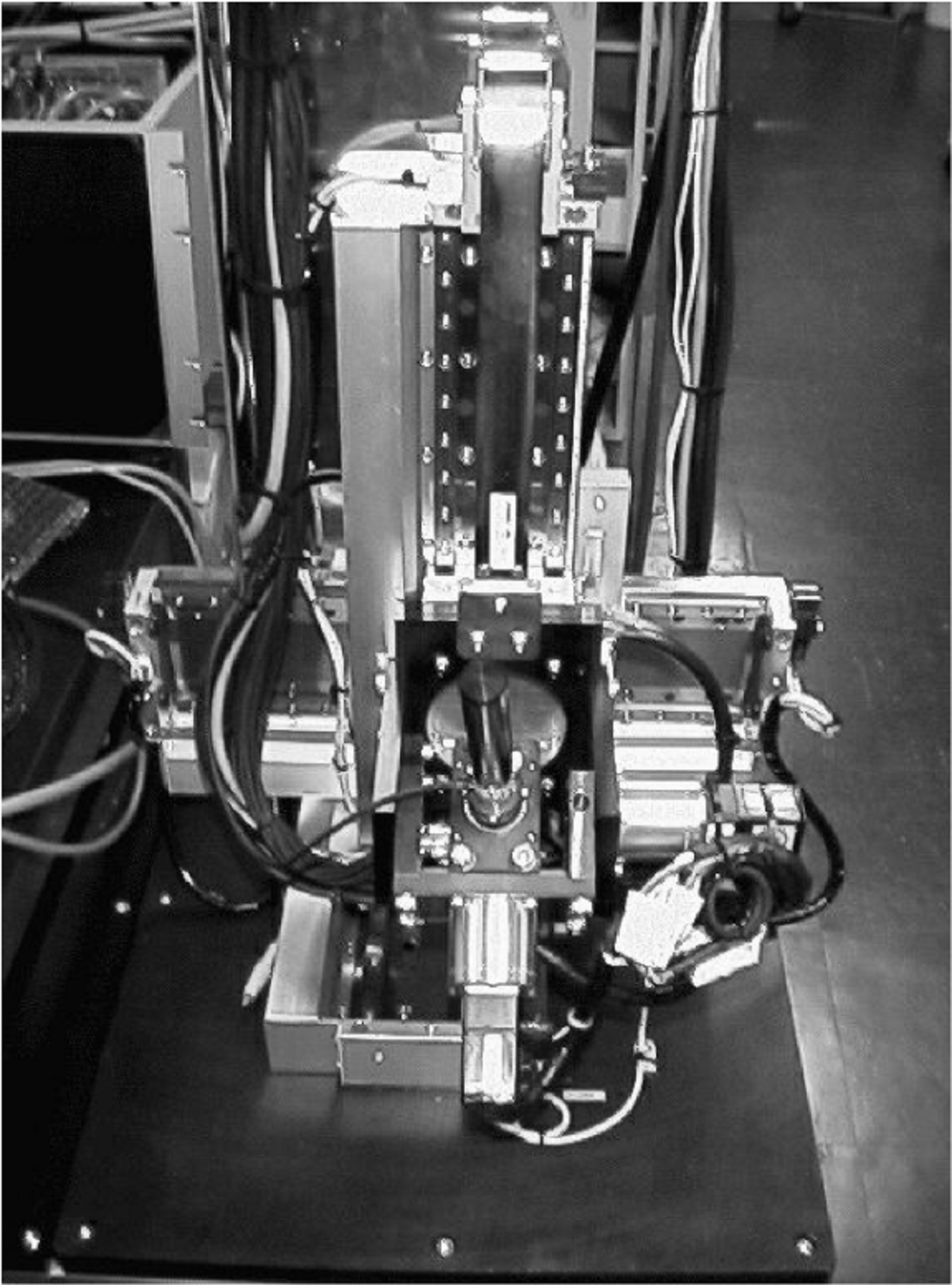
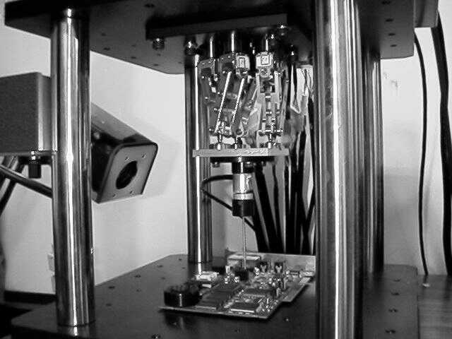
4.4.5.1. The Master Device of the micromanipulation system
The structure of master device is ought to be same as the slave device. However the parallel link structure has small workspace, which is not convenient for the human operator. That is why a serial link structure is applied to get large workspace, although it decreases accuracy and stiffness. The master device is stick-type device composed of 3 linear servo motors which realize 3 axis (X, Y, Z) parallel movement and 3 AC servo motors which realize rotation around each axis (, , ) [12] (see 4-17. ábra). It covers all 6 degrees of freedom of the slave device. The operator holds the master-stick in his hand and he can move and rotate it. The workspace is 340mmx340mmx340mm for linear movement, and the possible rotation is +/- 15 degrees for each axis. All degrees of freedom have force feedback.
4.4.5.2. The Slave Device of the micromanipulation system
As a slave device, a parallel link manipulator [13, 14, 15] was developed (see in 4-18. ábra), which has 6 degrees of freedom. In general, the parallel link structure has good features of precision and stiffness, although it has small workspace. This structure is fit for precise manipulation. It has 3 degrees of freedom for XYZ linear motion and 3 degrees of freedom for rotation of each axis. Its workspace is almost 30mmX30mmX30mm for linear motion and +/- 15 degrees for rotation. The positioning accuracy is 10 m. It is different from the well-known Stewart Platform structure [15], it has novel structure: Six links, which sprouted verticality from base table can expand and contract. Each two links of six links are combined into one by sublink. Ultimately, the end effector table is held by total 3 points (details in [13]). This manipulator is controlled by a PC (dual Pentium III 500MHz). Operating System is Real Time Linux (RT-Linux) in order to perform motor control with 2.5 kHz sampling time. Input-output using motor, rotary encoder, force sensor are performed by AD, DA, counter, DIO boards connected to an extended bus. As actuators, six AC servomotors of the same type are installed, and 1mm pitch ball screws are connected to each motor. The main drawback of this structure is the complex kinematics and dynamics with singular points as discussed in [13].
4.5. Animation of the operator’s hand wearing the sensor glove
Visual feedback is aimed at giving a quite real representation of the operator’s hand, and the program enables the user to wander it in full three-dimensional space.
The program was designed to run either locally in full simulation mode or over TCP/IP connection, such as Internet or Local Area Network. In simulation mode, the program can be used to represent all the motions of the human hand. To accomplish it, both anatomical and mathematical models were built up, and these models were implemented in OpenGL. The mathematical deduction uses the Denavit-Hartenberg notation, because it can be quite well applied both for hands and in OpenGL. The model uses several basic assumptions, these are:
The base coordinate frame is the same for all fingers. This is used for having a completely general case, where the fingertip coordinates are calculated with respect to a common frame of the wrist.
This common frame is considered to be at joint 0. This joint is used in order to have the possibility to extend the model at a later time if needed.
One finger contains three joints, the first has two degrees of freedom, the other two have only one, which means planar rotation. The position of the first joint is determined by a variable l0 ,which is the distance between the first, common coordinate frame and the first joint.
Along one finger, the value of diis 0, which means that the common normal line on the same line.
Along one finger the value of ai is the length of the link.
The twist angle is taken into account only at the base coordinate frame and at the first joint, since lateral movement of the finger is also considered.
It is important that coordinate frame 0 is the same for all fingers, and is a common reference to the whole hand. The individual i angles and l0 variables determine the exact position and orientation of the next frame of the next joint in each finger. Between the two frames di is just equal to the length of the link, l0. Since joint 0 is of the revolute type, q0 is 1 the relationship between the two joints is (4.1).
|
|
(4.1) |

In (4.1) A01is the 44 homogeneous transformation matrix between the two adjacent joints and Xsare position vectors in the respective coordinate frames.
|
|
(4.2) |
|
|
(4.3) |
As it was stated, in this case is 0º, which means that its cosine is 1 and its sine is 0. For the two joints d is taken to be 0 and a is the length of the link. Substituting these values simplifies the previous equation and yields to (4.4).
|
|
(4.4) |
Now the position and the orientation of the coordinate frame at joint 1 is received, further transformations can be carried out.
Now there is a general formula for calculating the position of the finger tip with reference to the common base coordinate frame. (4.3) shows this, and it is very similar to (4.1). Matrix T contains the position and orientation of the tip in the base coordinate system.
|
|
(4.5) |

It is useful to state that joint 2 has two transformation matrices and frames because of the two possible axis of rotation.
|
|
(4.6) |

where X15 is the position vector of the fingertip in its local co-ordinate frame.
The position and orientation of all five fingertips with respect to the common base frame (the wrist), is given by (4.7) as a function of joint angles.
|
|
(4.7) |

4.5.1. Grasping
4-20. ábra illustrates the transformations between finger-tip, contact and object coordinate frames [10]. Let us define homogeneous transformation matrices Ui R4x4 and Vi R4x4, where Ui transforms from the finger-tip coordinate frame Ti R4x4 to the contact frame Ci R4x4 and Vi R4x4 from the contact frame to the object frame Bi R4x4.The x- and y-axis of the contact coordinate frame Ci are tangents and the z-axis is perpendicular to the object surface curvature. (4-21. ábra). The transformation matrices i R6x6 and i R6x6 are defined such a way that i transforms finger-tip forces Tifi into forces Cifi in the contact coordinate frame and i transforms these to forces Bfi in the object reference frame B.
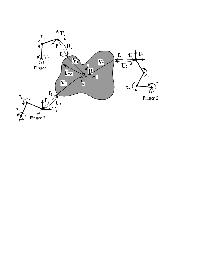
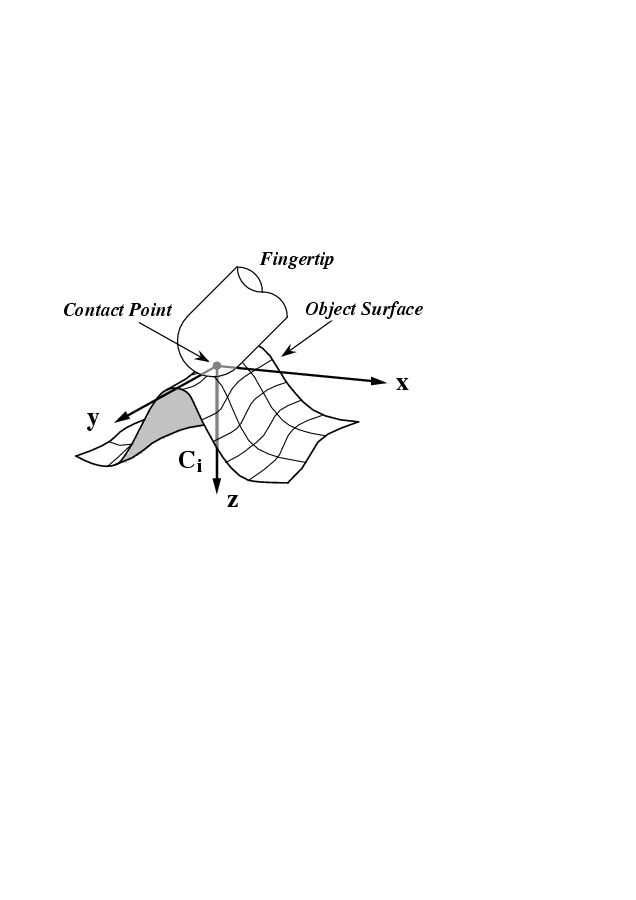
The relationship of coordinate transformations can be written as
|
Ci= Ti Ui B= Ci Vi= Ti Ui Vi Cifi =i Tifi Bfi=i Cifi=i i Tifi |
(4.8) |
where Ui, Vi are homogeneous transformations and i , i are force transformations [10]. The sensor glove has two types of sensor outputs, the torques actuated by the human operator R5x4 and the finger joint angle values R5x4. Ti are calculated from the forward kinematical equations using .
4.6. Overview of control modes
4.6.1. Basic Architectures
As it seen in 4-2. ábra, the communication takes place in two directions in a telemanipulation system. The controller with two directions for the control commands collectively referred as bilateral controller. Before the electrical master-slave system was developed, in order to realize force reflection, the traditional bilateral controlled master-slave system had been proposed since in 1952 (see in 4-22. ábra) [1] 4-23. ábra shows another traditional control approach for the master-slave system, which was introduced in 1954 [2]. The two position controllers control both the master and slave positions.
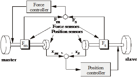
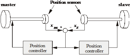
These basic architectures are often used as a starting point to design new controllers. Three main problems and some possible solutions are discussed here.
Nonlinear scaling (Virtual coupling impedance)
Time delay compensation of internet based telemanipulation
Friction compensation of master device
4.6.2. Nonlinear scaling (Virtual coupling impedance)
There are basically two approaches: linear and nonlinear scaling. In the case of linear scaling a single corresponding constant is used between the slave force/position and master force/position:
|
|
(4.9) |
where xs* and Fs* are the scaled values, p and p are the constants of position and force scale, respectively. In case of nonlinear scaling which is also called impedance scaling [14], forces are scaled independently with respect to their length scaling power relation as follows
|
|
(4.10) |
Where MV is the virtual mass, DV is the virtual viscosity constant and KV is the virtual stiffness. Note that this scaling method is similar to the concept of virtual impedance, which is widely used in the field of robot manipulators. Impedance scaling improves the performance, especially when the sizes or structures of the master and slave devices are different. The mechanical size has some correlation to its bandwidth. There are certain frequency and amplitude ranges, which are necessary for comfortable manipulation. The reaction force must be transformed into these ranges by the virtual coupling impedance. For example, in case of micro/nano manipulation, the reaction times of the micro/nano actuator and the micro/nano environment may be too fast for human tactile receptors. The reaction force must be slow down i.e. the high frequency components must be shifted to the lower frequency range with the help of virtual coupling impedance. In addition, the virtual coupling impedance behaves as a low pass filter in the communication channel. It can suppress the high frequency components, which can destabilize the system with time delay. In the other hand, it contradicts the requirements of ideal telepresence and transparency. In general, an impedance scaling may help avoiding instabilities and unreliable force feeling but the price, which must be paid for it is the loss of the degree of telepresence and transparency.
4.6.3. Time delay compensation of internet based telemanipulation
The efficiency of telemanipulation has been grown in the last few years. The application of the Internet gives new possibilities to the researcher [15]. The medium for data communication is the Internet in 4-1. ábra. It allows connecting places electronically that are thousands of miles apart. By combining network technologies with the capabilities of mobile robots, Internet users can discover and physically interact with places far away from them, creating opportunities in resources sharing, remote experimentation and long-distance learning. Burgard et al. [16] proposed an interactive museum tour guide robot for guiding the user to visit a museum. Simmons [17] presented an autonomous tour guide robot at Carnegie Mellon University. These tour guide robots have the capabilities of obstacle avoidance, self-referring, and path planning. Web users can control the autonomous robot through a web browser such as Netscape and Microsoft Internet Explorer, and click mouse on a map to assign the desired visiting position. Farzin and Goldberg [18] developed an interactive online lightbox system to provide users with the function of controlling the camera view for captured images. Stein [19] provided web users with a robot arm to paint a picture through a Java™-based user interface. Kosuge et al. [20] proposed the VISIT system using predictive strategy. Hirukawa and Hara [21] constructed a visual model robot arm to assist the teleoperation.
The main problem of Internet based Telemanipulation is the variable time delay. TCP/IP (Transport Control Protocol/Internet Protocol) is mainly used to stream data via Internet. It is a packet switched protocol. This means that the driver divides the data into packets, and sends the packets individually. The receiver tries to collect all the packets and rebuild the original data from the packets. A time delay always occurs when the signal extend from point A to point B. In addition, variable time delay is an immanent characteristic of a packet switched network. Variable time delay has two main reasons. One, the routes of the packets might be different on the network. Second, some packets might be lost. In this case, the receiver asks the driver to send the lost packet again and again. This time delay can destabilize a bilateral teleoperator system. The instability caused by time delay has been revealed by Ferrell [22] as early as 1965. Since that, various approaches for handling the problem of time delay [23] have appeared in the literature, like delay modeling and control system design [24], predictive displays and advanced operator interfaces [25], shared compliance control [26], impedance control [27], or supervisory control [28]. One possible solution for elimination the effect of time delay, namely virtual coupling impedance with position error correction method [29] is discussed in details. This control approach is an extension of the control approach by Otsuka et al [30]. Virtual coupling impedance is applied both at the operator and the remote site. An additional position correction loop is used to synchronize the two distant sites. This control approach is useful to compensate the effect of variable time delay, also appearing on the pocket switched computer network, like TCP/IP.
4.6.3.1. The Smith Predictor
The Smith Predictor is a classical configuration for time delay compensation [31]. Let the P(s) is a first order filter with transportation leg Td. The P0(s) is the model of theplant P(s) in which the time delay is eliminated
|
|
(4.11) |


There are two loops in 4-24. ábra. In the inner loop, a compensation signal v(t) contains a prediction of y(t). C0(s) is a PID controller.
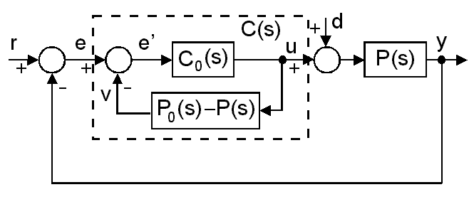
The closed loop transfer function is
|
|
(4.12) |
Notice, the transcendental term is eliminated in the characteristic equation of the closed loop transfer function. In practice, the perfect model P(s) is not known i.e. perfect elimination impossible, but the Smith predictor reduces the effect of time delay.
4.6.3.2. Wave variable approach
This approach is based on the passivity theory [32], which has close relationship to the Lyapunov stability. The passivity formalism represents a mathematical description of the intuitive physical concepts of power and energy. The basic idea behind passivity is to limit the input power flow such that it does not exceed the output power flow. If the power dissipation is zero, the system is called lossless. In case of a simplified telemanipulation, the operator moves a master device and its velocity vm is transmitted to the slave device, which is forced to follow the master movement, ideally vs= vm. The slave device contacts the remote environment and the reaction force Fs is transmitted back to the operator, who senses Fm=Fs. 4-25. ábra shows a simple telemanipulation with a constant time delay Td in the communication channel, where
|
vs(t)=vm(t-Td) Fm(t)=Fs(t-Td) |
(4.13) |
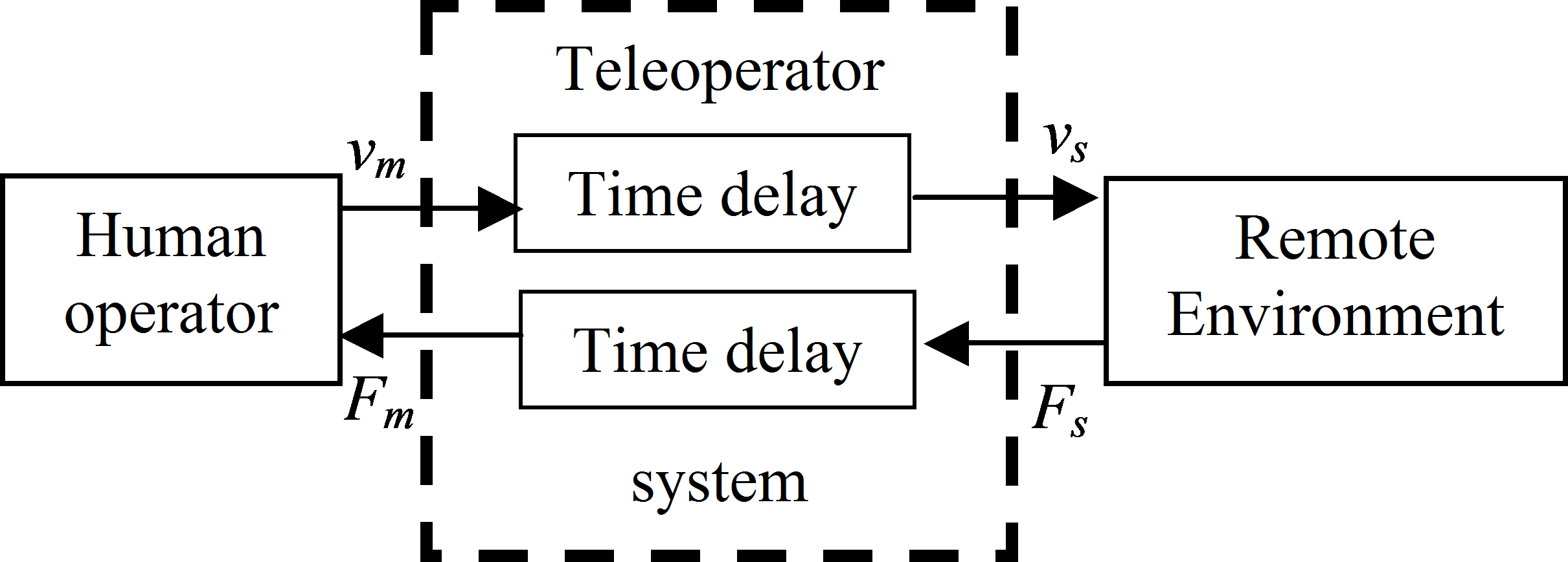
To handle the stability problem caused by the time delay, the bi-directional communication channel is considered as transmission line with a pressure type wave wV(t), a flow rate type wave wI(t) and a power P(x,t)= wV(x,t)wI(x,t), where x indicates that the wave variables must be measured at the same position of the. For stable operation, the transmission line must be passive, the dissipated energy must be non negative.
|
|
(4.14) |

where Pdiss is the power dissipation.
The trivial selection of wave variables (wI= vm and wV= Fs) does not lead to a passive transmission line. It highlights the source of the original problem. If the master velocity signal is sent and the slave force signal is received via Internet, the time delay may destabilize the operation of the telemanipulation system. To achieve a passive i.e. stable system, the “damping” or “leakage” of the transmission line must be increased. Introducing the following normalized wave transformation proposed in [33]:
|
|
(4.15) |


the transmission line becomes passive and lossless, which means the dissipated energy is zero. The velocity and force signal is transferred into wave variables before sending and they are retransferred after arriving (see in 4-26. ábra). A possible interpretation of (4.15) is that there are direct feedbacks from the velocity to the force at the master side and from the force to the velocity at the slave side.
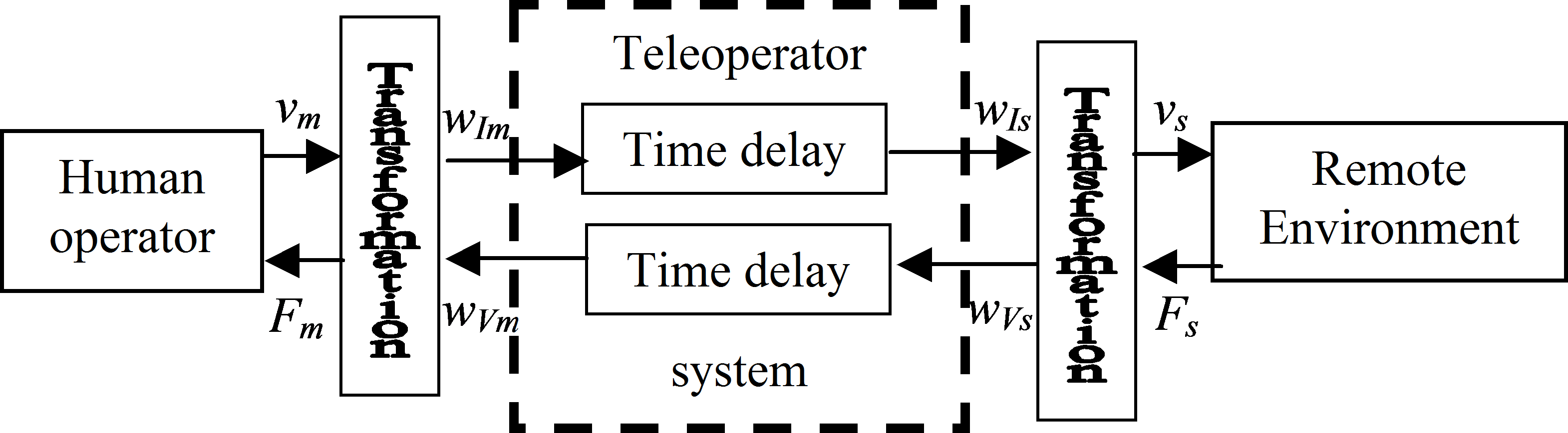
Mechanical impedance can be defined in the frequency domain.
|
|
(4.16) |

According to [36], perfect transparency can be ensured by perfect impedance matching. It can be interpreted as the reflected wave deteriorates the transparency. The terminating impedance of this transmission line includes the characteristics of the remote environment. For ideal transparency the frequency response of the remote environment must be known, and the transmission line has to be modified to mach it in the whole frequency domain. There is no such ideal solution but several papers are published to propose an optimal solution.
4.6.4. Friction compensation for master devices
The main problem is that the mechanism applied as a human interface device usually has a reasonable immanent friction. When the operator moves the master device, the friction might be too big to move it smoothly. Because of this additional force, the operator cannot feel, which force is exerted in remote environment and which force moves the master mechanism. The whole effect of the friction and the whole dynamics of the mechanic construction cannot be eliminated (since it would needed infinite input power) but it can be significantly reduced. The aim of the compensation is to make the system follow an ideal model with small friction. In other words, because of the compensation, the operator feels that it is very easy to move the master device.
The ideal model for a single joint:
|
|
(4.17) |

where u0 is the input current of the motor, which is proportional to the torque and f is the external torque. The state space variables: [rad] is angle position, [rad/sec] is the angular velocity.
|
|
(4.18) |
where the subscription “m” and “Δ” refer to the model and the difference between the model and the real parameters.
|
|
(4.19) |


|
|
(4.20) |


where Jm is the moment of inertia of rotor of DC motor, Dm is viscosity friction constant of DC motor and Km is the torque constant. The observer (model) equation:
|
|
(4.21) |
Since  , the Laplace transform of (4.21) is
|
|
(4.22) |
If the torques is considered as the input of the system the constant  is not necessary. Usually the following simplified, linearized reference model is selected for each degree of freedom of the master device
|
|
(4.23) |
where torque is the input and velocity is the output signal, Jm is the artificial inertia, Dm is the artificial viscous friction constant. The subscription m refers to the model. Parameters Jm and Dm must be small enough for comfortable manipulation but they must be big enough to avoid the undesirable motion (jitter).
4.6.4.1. Model Reference Adaptive Control based friction compensation
The ideal model with small friction is selected
|
|
(4.24) |

where  is the torque of the motor. The control law of the plant is defined as
|
|
(4.25) |

, where p is the input gain and q is the feedback gain. The closed loop transfer function is
|
|
(4.26) |
The closed loop system (4.26) behaves as the reference model (4.24), if
|
|
(4.27) |


Selecting the following Lyapunov function
|
|
(4.28) |
where  and
and  are the adaptation parameters. The Lyapunov stability criterion guarantees the global stability of the dynamic system (4.26), if
  is negative semidefinite, which can be ensured be the following adaptive law [17]:
|
|
(4.29) |
4.6.4.2. Sliding mode control based friction compensation
To compensate nonlinear friction force, sliding mode based friction observer will be introduced in this section. Consider the following model with external disturbances and uncertain parameters satisfying the so-called Drazenovic condition, written in the regular state equation form,
|
|
(4.30) |
where  and the bar
  refers to the nominal or desired (ideal) system matrices.
  and
and  are the respective uncertain perturbations and f(t)is an unknown, but bounded disturbance with bounded first time derivative with respect to time.
Now is defined as the uncertainties and the disturbance of the system.
|
|
(4.31) |
The second line of (4.30) can be rewritten by .
|
|
(4.32) |
According to [34],  is estimated by a discontinuous observer:
|
|
(4.33) |
whereis the discontinuous feedback. The goal of the design to find a feedback signal, denoted, such that the motion of the system (4.30) is restricted to belong the manifoldS.
|
|
(4.34) |
In sliding mode ( ),
), contains information on the system's parametric uncertainties and the external disturbance, which can be used for feedback compensation (compare (4.32) and (4.33)).
The simplest control law, which can lead to sliding mode, is the relay:
|
|
(4.35) |
If is in the range of B2 ( range (B2)), the ideal sliding mode occurs [35].
In the practice, there is no way to calculate the equivalent control veq precisely, but it can be estimated by a low pass filter for v as showed in 4-27. ábra. There are two loops in 4-27. ábra. The observer – sliding mode controller loop should be as fast as possible to achieve an ideal sliding mode. This is granted because this loop is realized in a computation engine in the recent application. The real system – compensator (consisting of Sliding Mode Controller and LPF) loop should be faster than the change of the disturbance. On the other hand, the smallest un-modeled resonant frequency of real system should be out of the bandwidth of that loop to avoid chattering.
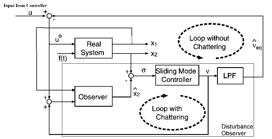
The robustness of continuous time sliding mode control is realized by the high-frequency switching of the discontinuous observer feedback signal . To adapt the sliding mode philosophy for a discrete time observer, the sampling frequency should be increased compared to Lumberger observer. If the switching frequency of the relay (4.35) is not enough high, might chatter around the manifold = 0. as shown in 4-28. , where Tk denotes the time of K-th
sampling. In case of discrete-time observer, the observer feedback signal may switch from +Mi and -Mi and vice versa resulting keq = 0 even if eq 0. The bigger the Miis, the bigger the chattering is. If Mi is smaller than the disturbances, it cannot eliminate the disturbances.
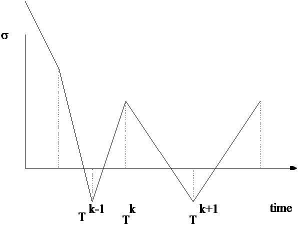
Applying the Lyapunov stability theory, let the positive definite Lyaponov function candidate is chosen in the following form:
|
|
(4.36) |

The observer feedback is chosen in such a way, that the derivation of the Lyaponov function meet the following condition:
|
|
(4.37) |

As it was proposed in [6,8], the condition (4.37) is satisfied if
|
|
(4.38) |

where D is a positive definite matrix.
|
|
(4.39) |
The observer feedback can be expressed from (4.38)
|
|
(4.40) |
The first term is responsible for the chattering free reaching of the sliding manifold, but it is 0, if the system in sliding mode. Since  is not known, the observer feedback must be estimated.
The discrete-time observer equation:
|
|
(4.41) |
where the discrete-time observer feedback estimated in the following form:
|
|
(4.42) |
where  , and D'=TD+I. It is noted, that the observer feedback (4.42) does not need additional LPF.
The advantage of this method that it does not need model inversion [16], which was the main problem in case of the inverted model, based disturbance observer.
Applying the above method for friction compensation of a single joint, the parameters are
|
|
(4.43) |


4.6.4.3. Friction Compensation Experience for sensor glove
The test system for tuning of the friction disturbance observer is shown in Fig. 4-29. The input signal of the system is the reference position. This signal is came from the angle sensor of main joint of the index finger. In this experimental three type of control pattern was introduced:
PD type controller without friction compensation
PID type controller without friction compensation and
PD type controller with friction compensation.
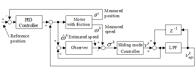
In order to emphasize the compensation capability of the method a simple PD controller is tested, which cannot eliminate the effect of the friction itself. The reference signal is a step change (0.2 rad). The external disturbance is also a step change, added to the motor input voltage but it lags 5s to the reference signal. Its absolute value is very big (12V) since it is equals to the max. input voltage. To avoid the saturation, it has an opposite sign that of the reference signal.
Fig. 4-30 shows the time functions of the reference and the measured positions. It is well known, that the PD controller can not eliminate the steady state error (see Fig. 4-30.). The same PD controller with compensation using disturbance observer can eliminate this error even when there is a quite big friction and load torque (see Fig. 4-30). In case of PID controller, the nonlinear characteristic of the friction causes a limit cycle. These results demonstrate the effectiveness of the sliding mode based disturbance observer, when external disturbance occurs.
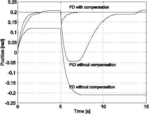
The friction compensator provides an additional compensation signal to any conventional closed loop controller and it improves its performance.
4.6.4.3.1. Free motion of the operator's index finger
The overall control system for free motion of the operator's index finger is shown in 4-31. ábra.. The input signal of the PID controller is zero, which means the sensor glove device follows the human hand. Free motion can be considered as a basic behavior of the haptic device. The operator is expected to feel no inertia and to move his finger freely. The friction of the device should be eliminated by control. In free motion, it is assumed that the error between the angle of the device and that of the human finger is detected by the torque sensor. There is a simple torque control loop, with a PID controller. Because of the nonlinear characteristics of the friction, it cannot be tuned well. The additional sliding mode based friction compensation may improve the performance significantly [13].
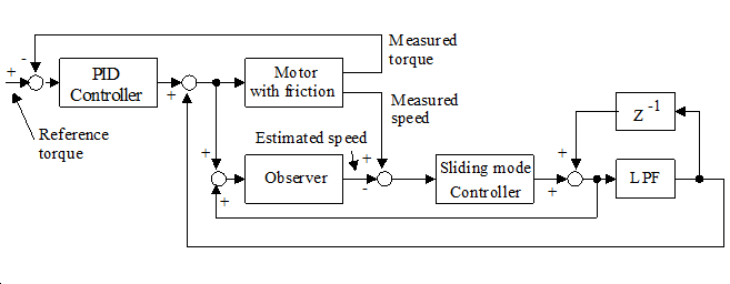
If motor is controlled in such a way that the strain gauge output voltage remains 0, the device follows the movement of the human finger and the operator cannot feel the friction force. Two controllers were compared namely a PID controller and a PID controller with disturbance compensation. The aim of these controllers is to nullify the torque measured by the strain gauge. In this experiment, the operator inserts his/her index finger in the device and moves only the root joint of the finger hand up and down during 10 seconds (see in Fig. 4-32. ábra). The upper plots are the angle of motor. The second graph in Fig. 4-32. ábra. shows the difference of the two methods clearly. The torque of the operator is small if the sliding mode disturbance observer is applied. The average torques of the finger joint are 0.009[Nm] (only PID) and 0.002[Nm] (PID with the sliding mode observer), respectively. Of course, the fatigue of the operator is not linear to the torque, the comforts of the operator significantly improved.
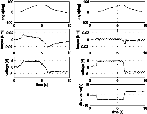
4.6.4.3.2. Virtual wall experiment
In this experiment the visual feedback is also used, so the first step was done to the telemanipulation. A virtual wall with constant elasticity is defined as in Fig, 4-33. ábra The virtual wall is -40 mm far from the operator’s palm. When the operator’s end of point finger reach the surface of the virtual wall’s position, the actuators of sensor glove give the force to finger. So the operator can feel the surface forces of the virtual wall. The sensor glove is a kind of dynamics interface between the operator, and the virtual reality. The operator four times touch the virtual wall. Each touch has different torque, as can seen on middle part of Fig, 4-33. ábra. The dashed line is the PID controller with disturbance observer, and the countinuous line is also a PID controller, but without disturbance compensation.
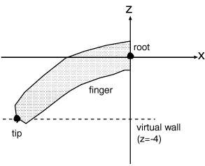
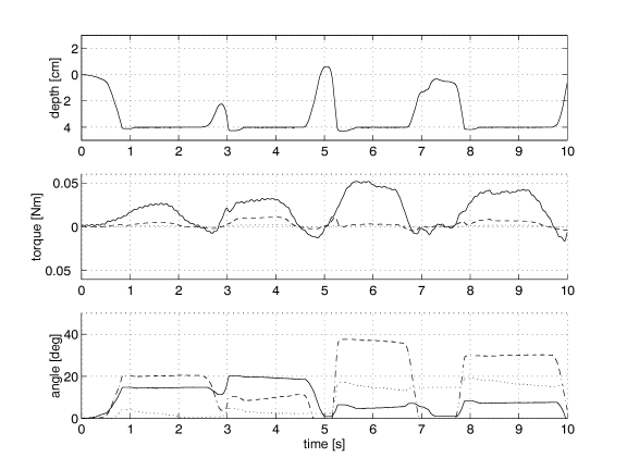
4.6.4.3.3. Visual Feedback of the operator
In the virtual wall experiment two computer was connected via memory mapping card. The memory mapping card give a common memory interval for the connected computers to share variables. In this experiment the joint angles and torques was shared between two computers. One computer is an IBM PC which is the computation engine for the sliding mode based disturbance observers for 20 degree of freedom. The other is an Indigo by Silicon Graphics. The challenge of Indigo is the visual interface for the operator. The Indigo contains the virtual reality and a virtual hand, what is like a reflection of the operator’s hand. When the operator moves his/her fingers the angle positions and
torques are shared with the Indigo. The indigo will draw a moving hand according to the operators hand position. When the virtual hand touch the virtual wall, forces interact between the hand and the wall. This forces are the base parameters for the control of sensor glove.
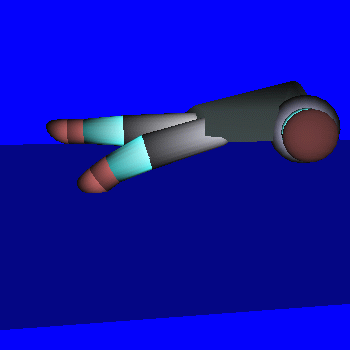
4.6.4.4. Friction Compensation Experience for the micro manipulation system
The whole effect of the friction and the whole dynamics of the mechanic construction cannot be eliminated (since infinite input power would be needed) but it can be significantly reduced. The friction force is measured approximately. In non-compensated case of axes Y, the friction force varied in the range of 20-30 N (see in Table 1).
|
Controller\Axis |
X |
Y |
Z |
|
Without Control |
10 [N] |
32 [N] |
14 [N] |
|
Classical MRAC |
0.05 [N] |
0.07 [N] |
0.05 [N] |
|
Sliding mode based MRAC |
0.001 [N] |
0.002 [N] |
0.005 [N] |
This force is too big for a smooth, comfortable operation. The aim of the compensation is to make the system follow an ideal model with small friction. In other words, because of the compensation, the operator feels that it is very easy to move the master joystick. Some tests were carried out to find when the operator feels the operation easy and comfortable. After these tests, the following linearized reference model is selected:
|
|
(4.44) |

where torque is the input and velocity is the output signal. According to the above model, the “artificial friction force” is only 0.1N with a constant speed of 2.5 m/s. A classical (see in 4-36. figure) and a sliding mode based (see in 4-37. ábra) model reference adaptive control methods are compared. The applications of these methods for friction compensation are published in [7] and [8].
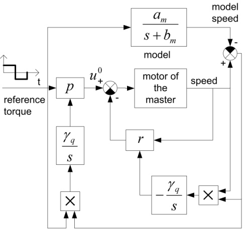
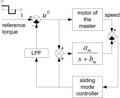
Because of the page limit axis X and Y are examined here. The reference signal is a squared pulse train with 0.1N amplitude and 0.4s period. The measurement results are shown in 4-38. figure and 4-39. figure. The friction of axis Y is significantly bigger. It is difficult to find an optimal adaptation parameter, which ensures fast adaptation but avoids the overcompensation. In overcompensated case, the joystick is moving randomly with 0 reference torque, because of the measurement noise. It is obvious that the bigger adaptation parameter means faster adaptation, but bigger possibility of random movement. The proposed Sliding Mode MRAC method seems to be more robust in our experimental environment.
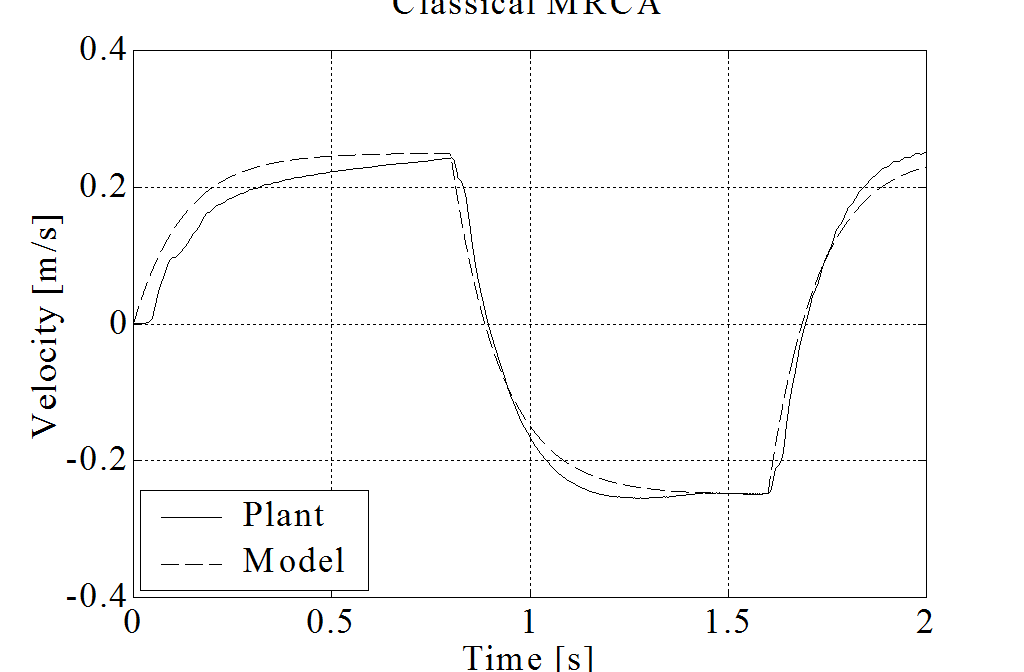

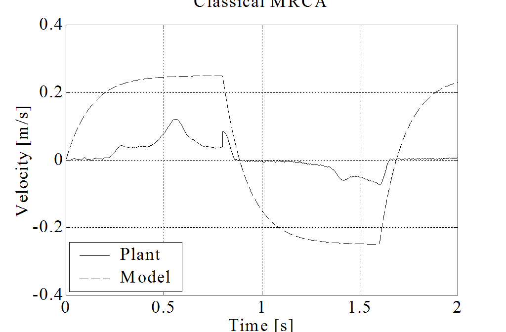
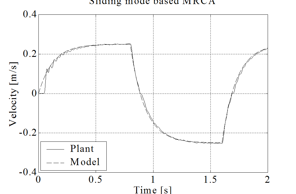
4.7. A complete application example: A handshake via Internet
A handshake via Internet is an interesting type of telemanipulation [29]. The task is to realize a handshake between two people at two different corner of the world. Let one be the one the operator and the other the far environment reacting to the operator (hand) movement. The master device will be a hand-shape device in the operator’s hand. The slave device is identical. When the operator grasps the master device (see in REF _Ref364272598 \h a and b), the master device transforms the movement and force to the slave device. The slave device gives this movement to the far environment (the other person’s hand). This person gives a reaction force and a movement to the slave device. This information is transmitted to the operator via master device. The handshake will be realized between two people far from each other. The main challenge is compensation of the time delay.
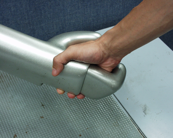
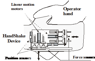
4.7.1. Virtual Impedance with Position Error Correction
Virtual Impedance with Position Error Correction (VIPEC) is based on the concept of the impedance control. VIPEC is composed of two major parts: a virtual impedance model (VI) and a position error correction part. The virtual impedance model generates a motion trajectory for a manipulator based on input forces and its dynamics. The position error correction part is added to decrease the position difference of the master and slave.
4.7.1.1. A. 1 Virtual Impedance
In the case of a 1 DOF linear motion manipulator, it is assumed that a virtual mass, Mv, is attached to a manipulator arm. This virtual mass is supported by a virtual damper, Dv, and a virtual spring, Kv. The structure of the VI is shown in 4-41. ábra.

When a force is applied to the virtual mass, the position of the virtual mass is modified according to the dynamics of VI. The dynamic equation of VI is as follow.
|
|
(4.45) |
where F(t) is the force detected at the virtual mass and x(t) is the displacement of the virtual mass. The transfer function of the VI acts as a second order low pass filter to convert force into displacement. Thus the displacement is always smooth even if the force contains high frequency components.
4.7.1.2. Position Error Correction
The structure of a teleoperator with time delay utilizing the VIPEC is illustrated in 4-42. ábra. The PEC part (the shaded part) is added to the original approach [30] in order to improve the response of the teleoperator by reducing the position error between the master and slave positions.
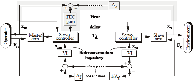
In 4-42. ábra, Fodenotes the force that an operator applies to the master arm, and Fe denotes the reflected force when the slave arm contacts with the environment. xm and xmrdenote the position and the reference position of the master arm. xsand xsr denote the position and the reference position of the slave arm. Td represents a delay time in data transmission between the two sites. Af is a scalar unit, which can be varied depending on the size ratio of the slave and the master.
Each VI generates the reference motion trajectory for each manipulator arm based on the sum of two forces: the force from its own site and the force received from the other site. The data transmission from one site to the other site is delayed by Td . The reference motion trajectory from VI is sent to a servo controller to control the position of the manipulator arm.
The control approach can be used for the master and the slave arms, which are different in size by appropriately adjusting Af and the parameters of each VI. For example, when the slave is a micro robot, which is smaller than the master.
The dynamic equation of VI at the operator site is
|
|
(4.46) |
The dynamic equation of VI at the remote site is
|
|
(4.47) |

Without loss of generality, Af =1 and both VIs have the same parameters. When the parameters of VI are appropriately determined, the system should remain stable. In the steady state, Fo is approximately equal to Fe when Kv is set to a low value, and the master and the slave positions should be identical. However, when time delay is present in the teleoperator, the control approach VI without PEC part causes the position error between the master and slave positions, since there is no comparison between these both positions. To reduce this position difference, the PEC part is added in order to make a closed loop system. Therefore the position error can be reduced. The slave position, delayed by Td, is transmitted to the master site and compared to the master position. The difference between the two positions is sent through the PEC gain, and then modifies the reference motion trajectory of the master arm.
Control model of the Handshaking device
4-43. ábra shows the control system diagram of the master-slave system inside the tele-handshaking system with VIPEC approach. The armature inductance, La of each motor is neglected. The two linear motion motors represented by the master block and the slave block can be modeled as simple DC-motors with the transfer function.
|
|
(4.48) |
where X and Ea are the Laplace transformed of motor shaft displacement and the applied armature voltage, Km is the motor gain constant, Tm is the motor time constant, and Kp is a constant to convert the angular displacement into displacement.
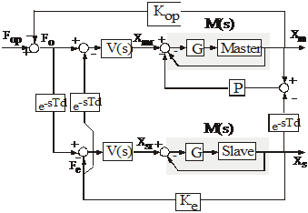
The servo controller is a proportional controller whose gain is G. The closed-loop transfer function of the manipulator arm and the controller is
|
|
(4.49) |
Gain P represents PEC gain. For simplicity, the environment is modeled by a spring with stiffness constant Ke. Therefore the dynamics of the spring interacting with the slave arm is modeled as follows.
|
Fe (t) = Ke xs(t), |
(4.50) |
where xs is the displacement of the spring. The dynamics of the operator including the dynamic interaction between the operator and the master arm is approximated by
|
|
(4.51) |

where Fop is the force generated by the operator's muscles. Mop, Bop and Kop denote mass, damper, and stiffness of the operator and the master arm respectively. Similarly to REF _Ref364274698 \h \* MERGEFORMAT , the displacement of the operator in (4.51) is represented by xm since it is also assumed that the operator is firmly grasping the master arm and never releases the master arm during the operation.
4.7.2. Experiment
Using the tele-handshake system, two human operators, operator A and operator B, shake hands with each other. When operator A tries to shake the hand of operator B by moving the master arm A, the slave arm A should move the same as the master arm A does. When the slave arm A contacts the palm of operator B, operator B can feel grasping force of operator A. Operator B also can grasp the virtual hand of operator A in the same way. Two operators succeeded to shake hands with each other and achieved force sensation through the tele-handshaking Device. Experimental results of simple VI and VIPEC methods are compared in 4-4. figure and 4-5. figure. In 4-4. figure, the time delay is negligible. The difference between the two methods is not significant. In both cases, the position of master and slave device are approximately the same. 4-5. figure illustrates the experimental results with 400 ms time delay. In both cases, the system is stable and the operators can feel grasping force. However, the position difference between the master and slave device is smaller in case of VIPEC method.
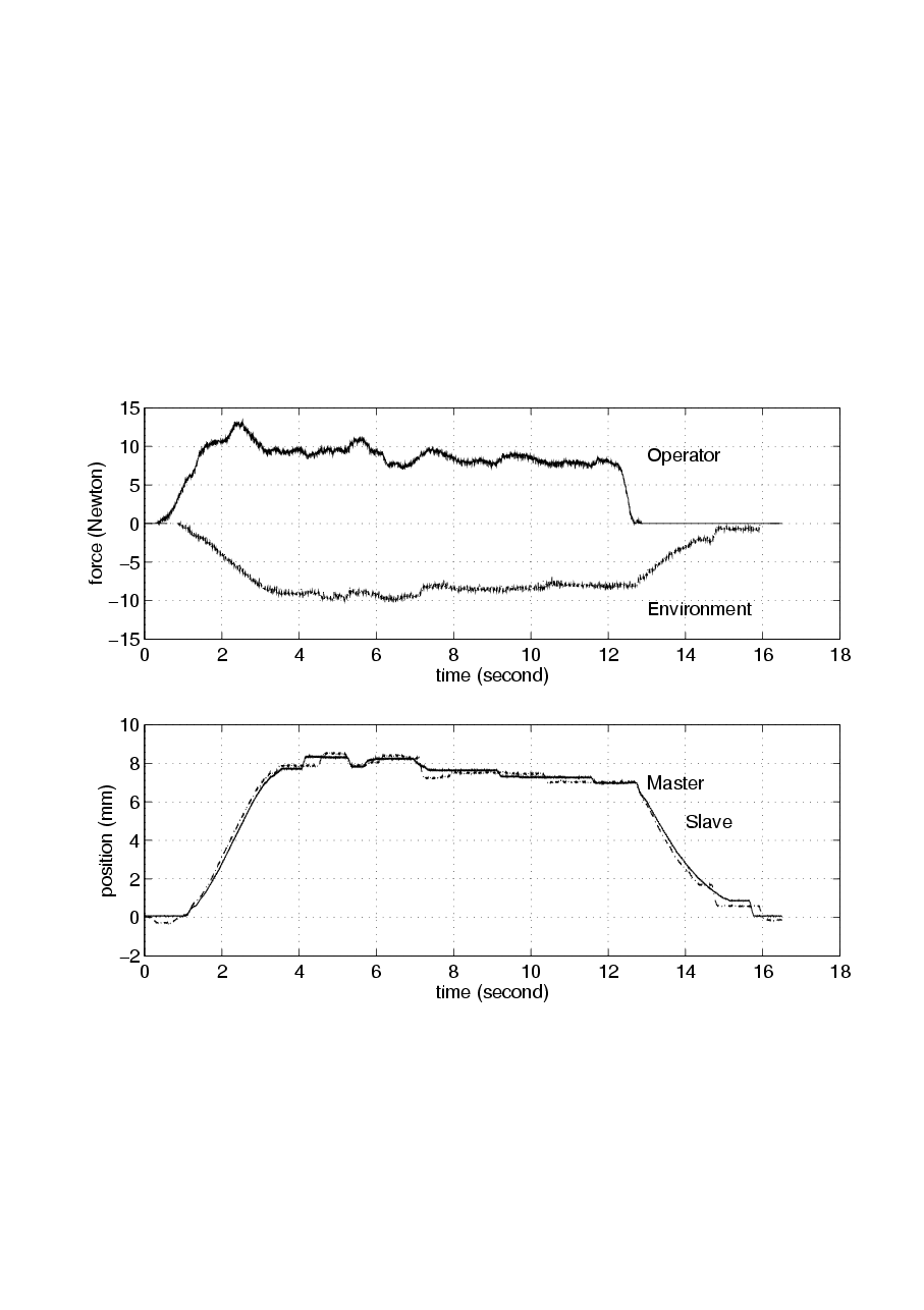
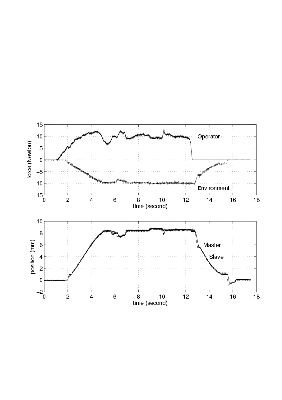
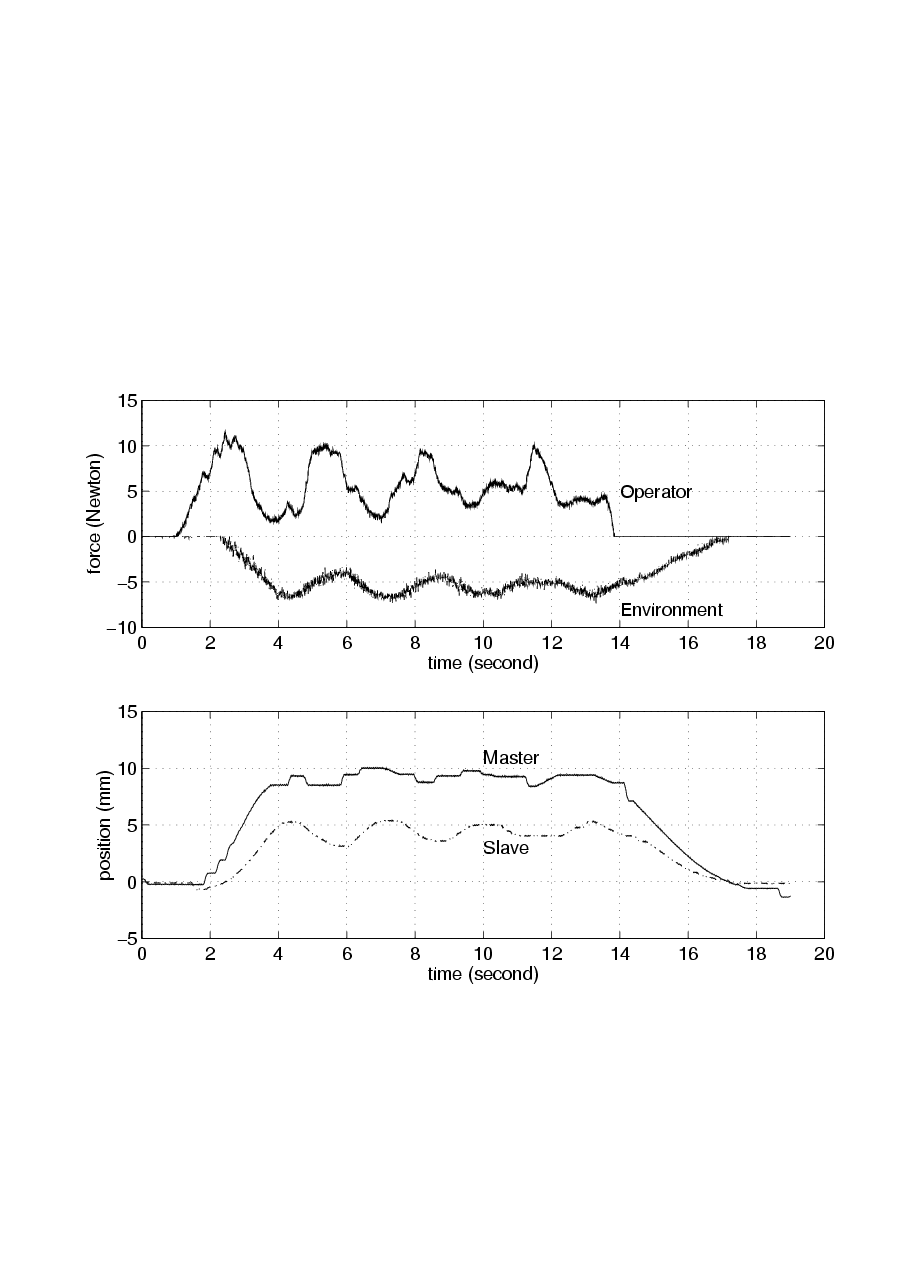
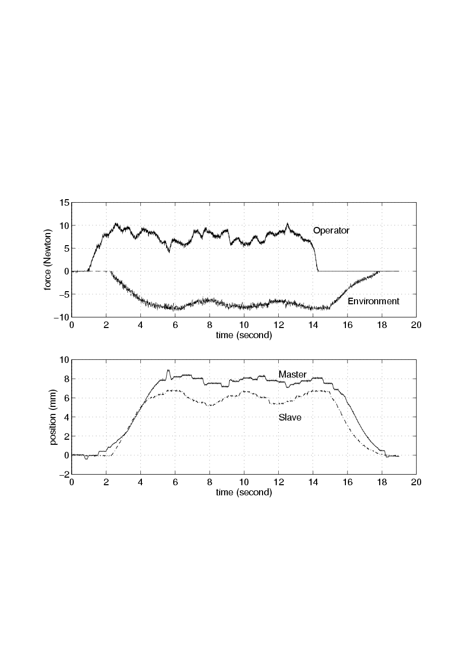
4.8. Conclusions for telemanipulation
The Internet based telemanipulation is a relatively new and attractive research field. It is fruitful ground for applying new and sophisticated control methods to eliminate the time delay and nonlinear friction force, which are the main challenges in this filed. Of course, the total elimination is impossible, but a stable operation may be achieved. This paper presented a promising method, namely Virtual Impedance method with Position Error Correction. The effectiveness of this method has been proved by measurement results of a tele-handshaking device.
4.9. References for telemanipulation
[1] T.B. Sheridan, “Telerobotics” Automatica, Vol. 25, No. 4, pp 487-507, 1989
R. C. Goertz and W. C. Thompson, „Electroically Controlled Manipulator” NUCLEONICS, Vol.12, No. 11, pp. 46-47, 1954.
[2] S. Lee, B. Bekey and A.K. Bejczy, “Computer Control of Space-borne Teleoperators with Sensory Feedback,” Proc. IEEE Int. Conf. On Robotics and Automation}, pp. 204-214, 1985.
[3] Barney Dalton, Ken Taylor: A Framework for Internet Robotics. Proceedings of IEEE/RSJ Int. Conf. on Intelligent Robots and Systems, WS2, pp. 15-22, 1998.
[4] S. Mizik, P. Baranyi, P. Korondi, and M. Sugiyama, “Virtual Training of Vector Function based Guiding Styles” Transactions on AUTOMATIC CONTROL and COMPUTER SCIENCE ISSN 1224/600X vol. 46(60) No.1 pp. 81-86. 2001.
[5] Handlykken M., Turner T., “Control systems analysis and synthesis for a six degree-of-freedom universal force-reflecting hand controller”, In proceedings of the IEEE Conference on Decision and Control, ‘80, vol 2, pp 1197-1205. 1980.
[6] Sheridan, T.B., “Telerobotic, Automation, and Human Supervisory Control” Cambridge, MA: The MIT Press, 1992.
[7] Burdea, G. and Coiffet, P.,“Virtual Reality Technology” New York: John Wiley & Sons, Inc, 1994.
[8] J. Dudragne, C. Andriot, R. Fournier and J. Vuillemey „A generalized bilateral control applied to master-slave manipulators” Proc of 20th Conference of International Society for Intelligent Research, pp. 435-442, 1989.
[9] Y. Kunii and H. Hashimoto, “Dynamic Force Simulator for Multifinger Force Display” IEEE trans. on IE, Volume 43, pp.74-
[10] Metin Sitti, Hideki Hashimoto: Two-Dimensional Fine Particle Positioning Using a Piezoresistive Cantilever as a Micro/Nano-Manipulator. IEEE International Conference on Robotics and Automation, pp. 2729-2735 1999.
[11] Thomas H.Massie, J.Kenneth Salisburg, ``The PhantomHaptic Interface: A Device for Probing Virtual Objects'', Proceedings of the 1994 ASME International Mechanical EngineeringCongress and Exhibition, Chicago, Vol. 55-1, pp.295-302
[12] Péter Korondi, Péter T. Szemes and Hideki Hashimoto, „Sliding Mode Friction Compensation for a 20 DOF Sensor Glove”, Transaction of ASME, Journal of Dynamic Systems, Measurement and Control, ISSN 0022-0434, December 2000, Vol. 122. P. 611-615.
[13] J. E. Colgate: “Robust Impedance shaping telemanipulation”. IEEE Transactions on Robotics and Automation, 9(4):373-384, Aug. 1993.
[14] Ren C. Luo, Tse Min Chen, Chih-Chen Yin: “Intelligent Autonomous Mobile Robot Control through the Internet”. ISIE 2000, Cholula, Puebla, Mexico, 2000 W.
[15] Burgard, A. Cremens, D. Fox, D. Hahnel, G. Lakemeyer, D. Schulz, W. Steiner, S. THRUN: “The Interactive Museum Tour-Guide Robot”. Proceedings of National Conference on Artificial Intelligence, pp. 11-18, 1998
[16] Reid Simmons: “Xavier: An Autonomous Mobile Robot on the Web”. Proceedings of IEEE/RSJ Int. Conf. on Intelligent Robots and Systems, WS2, pp. 43-48, 1998
[17] B. R. Farzin And K. Goldberg: “A Minimalist Telerobotic Installation on the Internet”. Proceedings of IEEE/RSJ Int. Conf. on Intelligent Robots and Systems, WS2, pp. 7-13, 1998
[18] M. R. Stein: “Painting on the World Wide Web: The PumaPaint Project”. Proceedings of IEEE/RSJ Int. Conf. on Intelligent Robots and Systems, WS2, pp. 37-42, 1998
[19] K. Kosuge, J. Kikuchi, K. Takeo: “VISIT: A Teleoperation System via Computer Network”. Proceedings of IEEE/RSJ Int. Conf. on Intelligent Robots and Systems, WS2, pp. 61-66, 1998
[20] H. HIRUKAWA And I. HARA: “The Web Top Robotics.” Proceedings of IEEE/RSJ Int. Conf. on Intelligent Robots and Systems, WS2, pp. 49-54, 1998
[21] R. Ferrell: “Remote Manipulation with Transmission Delay”. IEEE Transactions on Human Factors in Electronics, pp. 24-32, 1965
[22] Sukhan LEE, Hahk Sung LEE: “Advanced Telemanipulation under Time-delay”. SPIE OE/Technology ’92: Telemanipulator Technology, 1992
[23] A. K. Bejczy, W. S. Kim, S. C. Venema: “The Phantom Robot: Predictive Displays for Teleoperations with Time-delays”. IEEE International Conference on Robotics and Automation, pp. 546-551, 1990
[24] Won S. Kim, Blake Hannaford, Antal K. Bejczy: “Force-reflection and Shared Compliant Control in Operating Telemanipulators with Time-delay”. IEEE Transactions on Robotics and Automation, pp. 176-185, 1992
[25] Paul G. Backes: Multi-sensor Based Impedance Control for Task Execution. IEEE International Conference on Robotics and Automation, pp. 1245-1250, 1992
[26] W. R. Ferrell, T. B. Sharidan: “Supervisory Control of Remote Manipulation”. IEEE Spectrum, pp. 81-88, 1967
[27] Barney Dalton, Ken Taylor: “A Framework for Internet” Robotics. Proceedings of IEEE/RSJ Int. Conf. on Intelligent Robots and Systems, WS2, pp. 15-22, 1998
[28] S. Manorotkul and H. Hashimoto, “Virtual Impedance with Position Error Correction for Teleoperation with Time Delay,” Proc. 4th Int. Workshop on Advanced Motion Control}, Vol. 2, pp. 524-528, 1996.
[29] M. Otsuka, N. Matsumoto, T. Idogaki, K. Kosuge and T. Itoh, “Bilateral Telemanipulator System with Communication Time Delay Based on Forcesum-Driven Virtual Internal Model” Proc. IEEE Int. Conf. On Robotics and Automation, pp. 344-350, 1995.
[30] Smith O. J. M.: “A Controller to Overcome Dead Time”. Chem. Eng. Prog. Vol. 53, 217-219, 1959
[31] R. J. Anderson and M. W. Spong, “Bilateral Control of Teleoperators with Time Delay,” IEEE Trans. Automatic Control, Vol 34, pp. 494-501, 1989.
[32] Niemeyer, G., J-J.E. Slotine, “Stable Adaptive Teleoperation” IEEE trans. On Automatic Control, Vol. 16. No. 1. pp. 152-162. 1991.
[33] Young, K. D., “Manifold Based Feedback Design, Advances in Control and its Applications”, Lecture Notes in Control and Information Sciences, Springer-Verlag London, Tokyo, New York. 1995.
[34] Utkin, V. I., “Sliding Modes in Control and Optimization”, Springer-Verlag London, Tokyo, New York. 1992
[35] D. Lawrence, “Stability and Transpareny in Bilateral Teleoperation”, IEEE Transactions on Robotics and Automation, vol. 9, pp. 624-637, 1993.
Chapter 5. Holonomic based robot for behavioral research
Abstract— This chapter gives introspection to the concept of the MogiRobi – ethological model based autonomous robot. Technically, MogiRobi is a holonomic drive based mobile robot. Due to its ethological and cognitive info communication inspired design, it is able to visualize animal behaviors, high level interactions, and emotions. For evaluating high level interactions with the environment the robot works in an iSPACE (intelligent space). iSPACE is an environment, where external sensor network and distributed computing gives information for robot’s control algorithm. This development shows a viable trend for a novel methodology in the design of mobile service robots in the field of ethological behavior.
5.1. Introduction
There are many researches focused human robot interaction (HMI) in the last decade because service robots work at the same environment as people. This research takes in investigation of HMI from the ethological point of view, based on the 20,000 year old human-dog relationship [3]. The ethologists observing the dog’s behavior from the attachment point of view for the last fifteen years. Based on these observations a new type of artificial intelligent can be created that is able to attach to a specified owner.
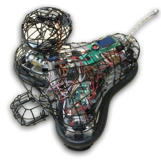
5.2. Concept
5.2.1. Etho-motor
The ethologic researchers were investigated the dog’s attachment behavior in the last 50 years. Today, the objective measurement of the attachment behavior is the Strange Situation Test (SST). Observing the dog’s behavior during several SST is the base input of an abstract emotional fuzzy model called etho-motor. This etho-motor keeps the high level control of MogiRobi.
5.2.2. iSPACE
The input information for the control algorithm is provided by iSPACE. ISPACE (Intelligent Space)[2] is an intelligent environment which provides both information and physical supports to humans and robots in order to enhance their performances. This performed by sensor network and distributed computing for preparing the rough sensor signals. During the behavioral experiments with the robot, the owner, a stranger and a toy take place in iSpace, see in Fig. 5-2. The operation depends on the behavior of the owner and the stranger.
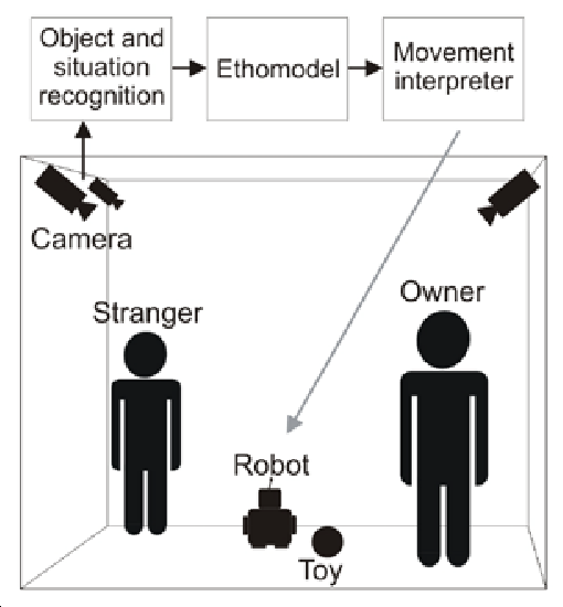
5.2.3. Behavior
Ethologically inspired research at the human-dog relationship and interaction suppose that dogs have evolved behavioral skills in the human environment. This social evolution increased the chances to survive in the anthropogenic environment. [5] Dogs use visual (e.g. tail, head and ear movement) and acoustic cues (e.g. barking, growling and squeaking) to express their emotions. Dogs also combine these methods to communicate with humans. Humans are able to recognize dogs' basic emotions without much specific experience. [6] In the view of our engineering methods, we do not provide an emotional model for the robot, but we provide a device to implement the model. The expression of the robot’s emotional behavior can be seen in Fig. 5-3 and Fig. 5-4 when the robot is sad or happy. We consider the analogy between the dog and the robot. We design human-robot interaction with the human-dog interaction analogy. Humans are able to recognize emotions on the robot from the main parameters of dog attitudes.
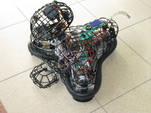
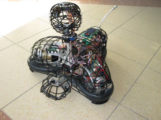
5.2.4. Drive system of the robot
At industrial environments non-holonomic robots are mostly appropriate for industrial tasks. But in case of social and service robots a further investigation is needed about the drive concept. The goal is to create a robot that can be easily accepted by people like a dog. In fact, the dog and the most of the animals have holonomic movement. The holonomic robots and dogs has an additional property that the moving and looking direction can be different during reaching a target on a non-straight trajectory (see Fig. 5-5). The moving and looking direction is always different in the case mentioned above. That is very a strange behavior if a non-holonomic driven robot looks away from it’s target during reaching it.
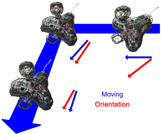
Based on this, we assume that the holonomic drive can be better for service robots for expressing emotional behavior by movement and looking during reaching a target. This holonomic property can be hardly achieved by a legged robot because of its high power consumption, and extensive engineering work needed for evaluating. Therefore the use of holonomic wheels (omni-wheels) is the compromise solution for MogiRobi.
5.3. Technical design of MogiRobi
5.3.1. The basement of the robot
Instead of legs the structure has a holonomical basement. It’s a new concept for mobile robot drive systems. The robot movement with legs would require much more power than rolling on wheels, and the movement with legs is more complicated and expensive. Smooth motion on legs would require complex control algorithms, expensive mechanical construction in more than one version. The most important factor at the design of the robot movement was the ability for motion in all planar degree of freedom. With omni-directional drive the robot can go to the reference position and orientation, in every direction at a time like a dog, not only forward and backward like differential drive or car like drive systems. Omni wheels are wheels with small discs (smaller wheels) around the circumference which are perpendicular to the rolling direction. (Fig. 5-8) This mechanical construction will result that the wheel can roll with full force, but also slide laterally with great ease. The three wheels are driven by three DC motors through driving gears, and belt transmissions. The robot can reach the 2 m/s top speed (7,2 km/h) in any direction. As Fig. 5-6 and Fig. 5-7 show, the motor shafts can be found around a circle swith the direction to the center point. The shafts are enclosing 120o. With this type of configuration we can get a 3 DoF holonomic system (x, y, rot z). The most of the overland animals can move in 3DoF: turning and moving in one direction in the same time. [4] The ordinary drive systems (steered wheels, differential drive) cannot perform this. The platform of MogiRobi can deliver 20 kgs with the maximal speed. It has about 0.25 kWatt DC motor power. It has 2 hours working time with one accumulator setup at normal use. There are incremental encoders on each motor shaft. From the signal of the incremental encoders and from the kinematics model of the robot we can calculate the x, y, rot z coordinates, during the path from point A to B. Also, we can plan the path between two relative reference points with interpolation. The animal type movement (acceleration, speed, path) could be implemented with the control algorithm in embedded system. The Motherboard on the robot basement can get relative position, orientation, absolute speed, acceleration references for the movement, and other peripheral references through Bluetooth port. The peripheral electronics can be connected via serial peripheral interface (SPI).
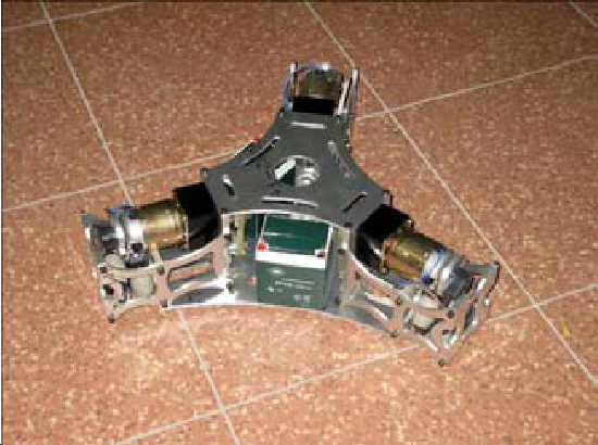
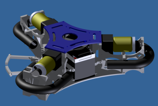
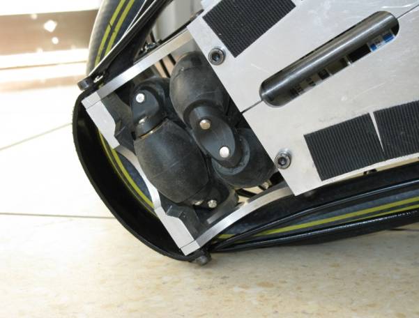
5.3.2. Body
The robot has a wired body, moved by two RC servos up and down. With this part the robot can behave like cats at aggressive behavioral attitudes.
5.3.3. Head
The head of the robot can be seen in Fig. 5-11, it has 4 DoF-s. It can be moved by the neck of the robot around the arc of the body. It connected to the body with a ball joint. The ball joint has 3 DoF-s (rot x, y, z). The head moves around the ball joint, with 3 RC servo drives. (Fig. 5-9 and Fig. 5-10) Two of these can be found on the neck for the rot x, y, and one in the head for the rot z DoF. (Where Z is the perpendicular axis.) The head has two ear, and eyelashes, also moved by compact servo drives.
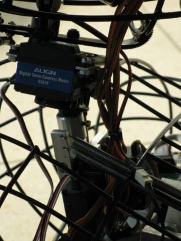
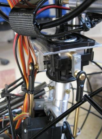
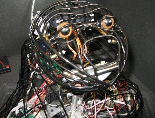
5.3.4. Gripper
The gripper can be seen in Fig. 5-12 it has a very important role when we play with the robot. The robot can fetch a ball with it.
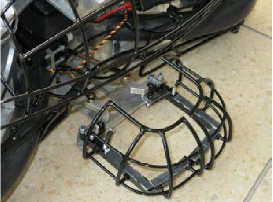
5.3.5. Tail
The tail has an important role at the visualization of the emotions. The mechanical construction of the tail can be seen in REF _Ref386997877 \h and Fig. 5-14 One servo drive moves the plastic tail through two wires. The tail was bended to the body with springs. The oscillating mechanical system for the wagging movement is excited by a DC servo drive. The damping of the system is negligible. With the test of several springs and control algorithms we could tune the system for acting like animal tail movements. These small factors are very important at the acceptance of the robot for children, elders, etc.
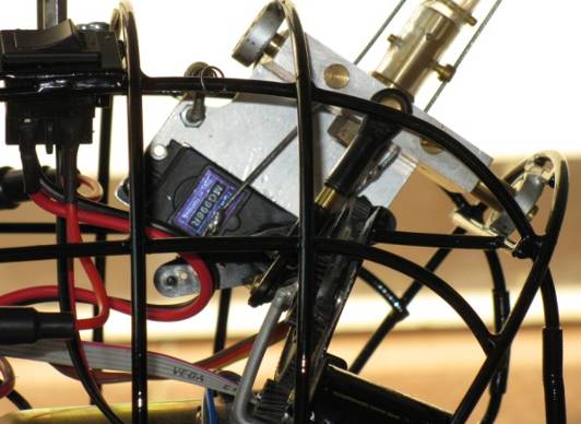
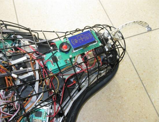
5.3.6. Control and power electronics
Each control board has one processor. The first is a simple 8-bit RISC Xmega processor from Atmel. () It can handle the communication with the server via Bluetooth. It also handles the motor control loop and the high level position calculation. It can send the reference angle of the servos to the servo board and handles 3 encoder channels for odometry. The servo control board can be seen on figure 17, it has 15 output channels for compact RC servos. In case of RC servos it is very important to use isolated power supply. The servo control board provides PWM signals for the RC servo drives. The servo drives have strongly limited accelerations for eliminating transient disturbances during movement. All servo trajectories calculated with low symmetrical acceleration profile, giving a smooth motion profile for the robot. The nominal power parameters of the PWM amplifier board are three times 24V/10A. We are using special automotive compatible ICs with current feedback, over current sense, and also a temperature sense. On the back of the robot we can found an LCD with control buttons, see figure 18. We can choose between the control methods. It can run self-test, or check the information, battery states.
The robot can be in play mode, where it gets the control commands from an external PC via it’s Bluetooth interface. At jogging mode, we can control the robot with the buttons. At self-test, the robot checks all of the peripheries, and servo drives.
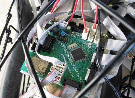
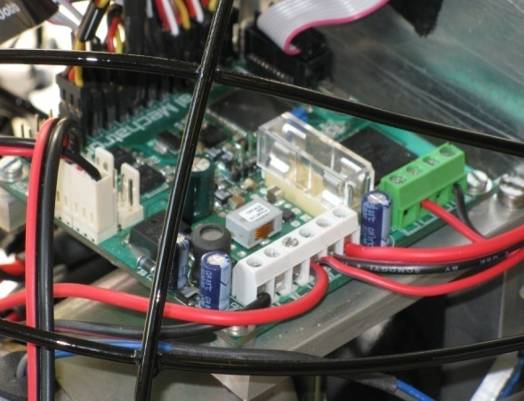
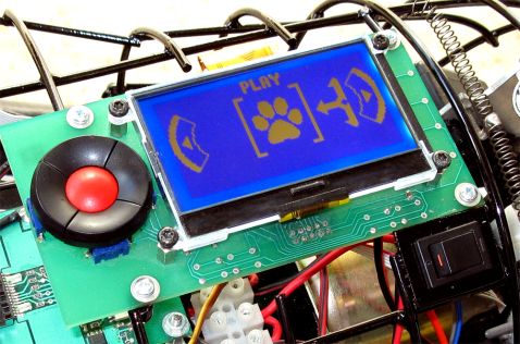
5.4. Conclusion
The goal of this paper was to suggest mechanical and control methods for a social robot in the iSpace conception. The control methods could be implemented, and tested in different situations. MogiRobi controlled with simple orders from the fuzzy logic system and worked at the iSpace conception with promising results. It is an easily built and well designed adaptable structure for many application areas at social robotics. The robot can cooperate with dogs and humans also. At the scenarios the emotions of the robot always recognized. It’s proved that the mechanical and control methods of MogiRobi were appropriate for Human-Robot, Dog-Robot interaction. The suggested mechanical structure was worked successful during emotion recognition, and cognitive communication.
Chapter 6. Fuzzy automaton for describing ethological functions
This chapter presents an ethologically inspired model realized with a fuzzy rule interpolation fuzzy automaton (introduced in REF _Ref366247252 \r \h , REF _Ref366247254 \r \h , REF _Ref366252238 \r \h and REF _Ref366247256 \r \h ). First, the ethological inspiraton for human-robot interaction is presented, after that a brief overview on behaviour-based control, then some words on fuzzy automata can be found. After introducing the necessary prerequisites, the ethological test procedure, the suggested structure of the model is described in details. Some samples from the rule bases of the fuzzy automaton along with example simulation executions are described.
6.1. Ethologically inspired Human-Robot Interaction
In recent years there has been an increased interest in the development of Human-Robot Interaction (HRI). Researchers have assumed that HRI could be enhanced if these intelligent systems were able to express some pattern of sociocognitive and socioemotional behaviour (e.g. REF _Ref361667391 \r \h \* MERGEFORMAT ). Such approach needed an interaction among various scientific disciplines including psychology, cognitive science, social sciences, artificial intelligence, computer science and robotics. The main goal has been to find ways in which humans can interact with these systems in a ‘natural’ way. Recently HRI has become very user oriented, that is, the performance of the robot is evaluated from the user’s perspective. This view also reinforces arguments that robots do not only need to display certain emotional and cognitive skills but also showing features of individuality. Generally however, most socially interactive robots are not able to support long-term interaction with humans, and the interest shown toward them wears out rapidly.
The design of socially interactive robots has faced many challenges. Despite major advances there are still many obstacles to be solved in order to achieve a natural-like interaction between robots and humans. The ‘uncanny valley’ effect: Mori REF _Ref361656179 \r \h \* MERGEFORMAT assumed that the increasing similarity of robots to humans will actually increase the chances that humans refuse interaction (will be frightened from) very human-like agents. Although many take this effect for granted only little actual research was devoted to this issue. Many argue that once an agent passes certain level of similarity, as it is the case in the most recent visual characters in computer graphics, people will treat them just as people REF _Ref361667499 \r \h \* MERGEFORMAT . However, in the case of 3D robots, the answer is presently less clear, as up do date technology is very crude in reproducing natural-like behaviour, emotions and verbal interaction. Thus for robotics the uncanny valley effect will present a continuing challenge in the near future.
In spite of the huge advances in robotics current socially interactive systems fail both with regard to motor and cognitive capacities, and in most cases can interact only in a very limited way with the human partner. This is a major discrepancy that is not easy to solve because there is a big gap between presently available technologies (hardware and software) and the desire for achieving human-like cognitive and motor capacities. As a consequence recent socially interactive robots have only a restricted appeal to humans, and after losing the effect of novelty the interactions break down fast.
The planning and construction of biologically or psychologically inspired robots depends crucially of the current understanding of human motor and mental processes. However, these are one of the most complex phenomena of life. Therfore it is certainly possible that human mental models of abilities like ‘intention’, ‘human memory’ etc., which serve at present as the underlying concepts for control socially interactive robots, will be proved to be faulty.
Because of the goal of mimicking a human, socially interactive robots do not utilize more general human abilities that have evolved as general skills for social interaction. Further, the lack of evolutionary approach in conceptualizing the design of such robots hinders further development, and reinforces that the only goal in robotics should be the produce ‘as human-like as possible’ agents.
In order to overcome some of the challenges presented above ethologically inspired HRI models can be applied. The concept of ethologically inspired HRI models allows the study of individual interactions between animals and animals and humans. This way of handling Human-Robot Interaction is based on the concept that the robot acts like an animal companion to human. According to this paradigm the robot should not be molded to mimic the human being, and form human-to-human like communication, but to follow the existing biological examples and form inter-species interaction. The 20.000 year old human-dog relationship REF _Ref361667925 \r \h \* MERGEFORMAT is a good example for this paradigm of the HRI, as interaction of different species. One good reason of this approach in HRI is the lack of the ‘uncanny valley’ effect REF _Ref361656179 \r \h \* MERGEFORMAT , i.e. there is no need to buit robots which have any similarities to humans.
Such robots do not have to rely on the exact copy of human social behaviour (including language, etc.) but should be able to produce social behaviours that provide a minimal set of actions on which human-robot cooperation can be achieved. Such basic models of robots could be improved with time making the HRI interaction more complex.
In ethological modeling, mass of expert knowledge exists in the form of expert’s rules. Most of them are descriptive verbal ethological models. The knowledge representation of an expert’s verbal rules can be very simply translated to the structure of fuzzy rules, transforming the initially verbal ethological models to a fuzzy model. On the other hand, in case of the descriptive verbal ethological models, the ‘completeness’ of the rule-base is not required (thanks to the descriptive manner of the model), which makes implementation difficulties in classical fuzzy rule based systems. For that reason for fuzzy modell we use low computational demand Fuzzy Rule Interpolation (FRI) methods like FIVE REF _Ref385680017 \r \h . The application of FRI methods fits well the conceptually sparse rule-based (‘incomplete’) structure of the existing descriptive verbal ethological models.
The main benefit of the FRI method adaptation in ethological model implementation is the fact, that it has a simple rule-based knowledge representation format. Because of this, even after numerical optimization of the model, the rules remain ‘human readable’, and helps the formal validation of the model by the ethological experts. On the other side due to the FRI base, the model has still low computational demand and fits directly the requirements of the embedded implementations.
For implementing ethologically inspired HRI models the classical behaviour-based control structure is suggested, described in the followings.
6.2. Behaviour-based control
The main building blocks of Behaviour-based Control (BBC, a comprehensive overview can be found in REF _Ref358152640 \r \h ) are the behaviour components themselves. The behaviour components can be copies of typical human or animal behaviors, or can be artificially created behaviours. The actual behaviour response of the system can be formed as one of the existing behaviour component, which gives the best match to the actual situation, or a fusion of the behaviour components based on their suitability for the actual situation. Encoding the behaviour components can be realized with e.g. simple reflexive agents, which assign an output response to each input situation.
In case when more than one behaviour components are simultaneously competing for the same ‘actuator’ the aggregation or selection of the behaviour components is necessary. Handling multiple behaviour components in a BBC system can be done in two ways. The first is the competitive way, when the behaviour components are assigned with priorities, and the behaviour component with the highest priority takes precedence, while the behaviours with lower priorities are simply ignored. The second is the cooperative way when the outputs are fusioned based on various criteria.
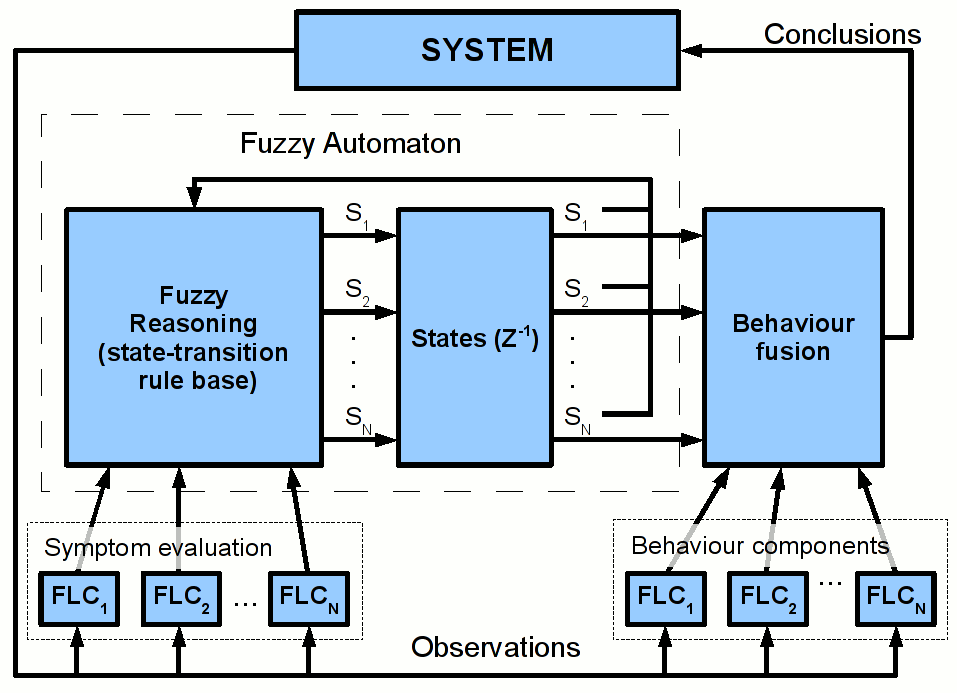
This structure has two main tasks. The first is a decision of which behaviour is needed in an actual situation, and the levels of their necessities in case of behaviour fusion. The second is the way of the behaviour fusion. The first task can be viewed as an actual system state approximation, where the actual system state is the set of the necessities of the known behaviours needed for handling the actual situation. The second is the fusion of the known behaviours based on these necessities. In case of the suggested fuzzy behaviour based control structures both tasks are solved by FRI systems. If the behaviours are also implemented on FRI models, the behaviours together with the behaviour fusion modules form a hierarchical FRI system.
The application of FRI methods in direct fuzzy logic control systems gives a simplified way for constructing the fuzzy rule base. The rule base of a fuzzy interpolation-based model, is not necessarily complete, it could contain the most significant fuzzy rules only without risking the chance of having no conclusion for some of the observations. The model always gives a usable conclusion even if there are no rules defined for the actual observations. In other words, during the construction of the fuzzy model, it is enough to concentrate on the main actions (rules could be deduced from the others could be intentionally left out from the model, radically simplifying the rule base creation, saving time consuming work.).
For demonstrating the main benefits of the FRI model in behaviour-based control, here the focus is only on the many cases most heuristic part of the structure, on the behaviour coordination. The task of behaviour coordination is to determine the necessities of the known behaviours needed for handling the actual situation.
In the suggested behaviour-based control structure for achieving the decision related to the relevance of the behaviour components this work adapts the concept of the finite state fuzzy automaton REF _Ref361677815 \r \h \* MERGEFORMAT (see Fig. 6-1 and the next chapter for more details), where the state of the finite state fuzzy automaton is the set of the suitabilities of the component behaviours. This solution is based on the heuristic, that the necessities of the known behaviours for handling a given situation can be approximated by their suitability. And the suitability of a given behaviour in an actual situation can be approximated by the similarity of the situation and the prerequisites of the behaviour. (Where the prerequisites of the behaviour is the description of the situations where the behaviour is applicable). This case instead of determining the necessities of the known behaviours, the similarities of the actual situation to the prerequisites of all the known behaviours can be approximated.
The system consists (see Fig. 6-1) of not only the fuzzy automaton but the behaviour fusion component and various component behaviours implemented on fuzzy logic controllers (FLC). The state variables characterize the relevance of the component behaviours. The state-transition rule base of the automaton applies fuzzy rule interpolation for state-transition evaluation. The previous states are fed back to the automaton and the conclusion given by the automaton is used as weights in the behaviour fusion component for determining the final conclusion of the BBC. The conclusion of the fuzzy automaton will be the new system state for the next step of the behaviour fusion. The behaviour fusion component can be also implemented by fuzzy reasoning (e.g. using fuzzy rule interpolation), or simply as a weighted sum. The symptom evaluation (from the terminology of fault classification) components provide a kind of preprocessing for the automaton based on the gathered observations. These components also can employ FRI techniques.
Therefore the first step of the system state approximation is determining the similarities of the actual situation to the prerequisites of all the known behaviours. The task of symptom evaluation is basically a series of similarity checking between an actual symptom (observations of the actual situation) and a series of known symptoms (the prerequisites – symptom patterns – of the behaviour components). These symptom patterns are characterizing the systems states where the corresponding behaviours are valid. Based on these patterns, the evaluation of the actual symptom is done by calculating the similarity values of the actual symptom (representing the actual situation) to all the known symptoms patterns (the prerequisites of the known behaviours). There are many existing methods for fuzzy logic symptom evaluation. For example fuzzy classification methods e.g. the Fuzzy c-Means fuzzy clustering algorithm REF _Ref361758798 \r \h can be adopted, where the known symptoms patterns are the cluster centers, and the similarities of the actual symptom to them can be fetched from the fuzzy partition matrix. On the other hand, having a simple situation, the fuzzy logic symptom evaluation could be an FRI model too.
One of the main difficulties of the system state approximation is the fact, that most cases the symptoms of the prerequisites of the known behaviours are strongly dependent on the actual behaviour of the system. Each of the behaviours has its own symptom structure. In other words, for the proper system state approximation the approximated system state is needed itself. A very simple way of solving this difficulty is the adaptation of fuzzy automaton. This case the state vector of the automaton is the approximated system state, and the state-transitions are driven by fuzzy reasoning (‘Fuzzy Reasoning (state-transition rule base)’ on Fig. 6-1), as a decision based on the previous actual state (the previous iteration step of the approximation) and the results of the symptom evaluation.
6.3. Fuzzy automaton
As mentioned previously, the structure of the proposed model follows the behavior-based control concept REF _Ref358152640 \r \h , i.e. the actual behavior of the system is formed as a fusion of the known component behaviors appeared to be the most appropriate in the actual situation. For behavior coordination in the applied model the concept of the ‘Fuzzy Automaton’ is adapted. Numerous versions and understanding of the fuzzy automaton can be found in the literature (a good overview can be found in REF _Ref286655753 \r \h ). The most common definition of Fuzzy Finite-state Automaton (FFA, summarized in REF _Ref286655753 \r \h ) is defined by a tuple (according to REF _Ref363657503 \r \h , REF _Ref286655753 \r \h and REF _Ref288780404 \r \h ):
|
|
(6.1) |
where Q is a finite set of states, Q={q1,q2,...,qn}, Σ is a finite set of input symbols, Σ={a1,a2,...,am},  is the (possibly fuzzy) start state of
  , Z is a finite set of output symbols, Z={b1,b2,...,bn},
  is the fuzzy transition function which is used to map a state (current state) into another state (next state) upon an input symbol, attributing a value in the fuzzy interval [0,1] to the next state, and
  is the output function which is used to map a (fuzzy) state to the output.
Extending the concept of FFA from finite set of input symbols to finite dimensional input values turns to the following:
|
|
(6.2) |
where S is a finite set of fuzzy states,  , X is a finite dimensional input vector,
  ,
,  is the fuzzy start state of
  , Y is a finite dimensional output vector,
  ,
,  is the fuzzy state-transition function which is used to map the current fuzzy state into the next fuzzy state upon an input value, and
  is the output function which is used to map the fuzzy state and input to the output value. See e.g. on Fig. 6-2.
In case of fuzzy rule based representation of the state-transition function  , the rules have
  dimensional antecedent space, and n dimensional consequent space. Applying classical fuzzy reasoning methods, the complete state-transition rule base size can be approximated by the following formula:
|
|
(6.3) |

where n is the length of the fuzzy state vector S, m is the input dimension, i is the number of the term sets in each dimensions of the state vector, and j is the number of the term sets in each dimensions of the input vector.
According to (6.3) the state-transition rule-base size is exponential with the length of the fuzzy state vector and the number of the input dimensions. Applying FRI methods for the state-transition function fuzzy model can dramatically reduce the rule base size. See e.g. REF _Ref358152171 \r \h , where the originally exponential sized state-transition rule base of a simple heuristical model turned to be polynomial thanks to the FRI.
In case of direct application of the suggested FRI based Fuzzy Automaton for behavior-based control structures, the output function  can be decomposed to parallel component behaviors and an independent behavior fusion. In this case the structure of the above introduced fuzzy automaton can turn to a very similar form as it is expected in behavior-based control (see Fig. 6-3 and Fig. 6-1). Some more details of the model implementation can be found in REF _Ref366247252 \r \h , REF _Ref366247254 \r \h and REF _Ref366247256 \r \h .
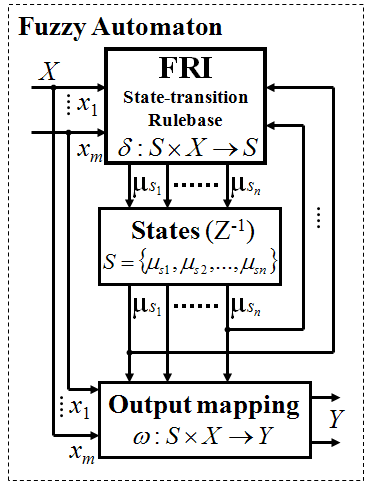
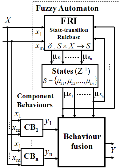
6.4. Simulation of the ‘Strange Situation Test’ (SST)
The ethological test procedure presented here has been developed for studying the affiliative relationship between a dog and its owner. The procedure is made up from seven episodes, each lasting 2 minutes, where the dog is in different situations: first with the owner, then with a stranger, or alone (according to a pre-defined protocol). Through the test, the dog’s behavior is evaluated mainly focusing on dogs’ responses related to their proximity seeking with the owner REF _Ref307389263 \r \h .
In the first episode of the test, the dog and the owner are in the test room. First the owner is passive, and then he/she stimulates playing. The second episode is where the stranger comes into the room and starts to stimulate play with the dog. Then the owner leaves the room, so in the third episode the dog is separated from the owner; the stranger tries to play with the dog then sits for a while and offers petting. The owner comes back in the beginning of the fourth episode, this is the first reunion. Meanwhile the stranger leaves the room and the dog is with the owner for two minutes. Then the owner also leaves, so in the fifth episode the dog is alone in the room. In the next episode the stranger returns and tries to stimulate playing or comfort the dog by petting it. The returning of the owner marks the beginning of the last episode. The stranger leaves the room, the owner interacts with the dog for two minutes and the test ends.
During evaluation, ethologists record pre-defined behavioral variables for describing the dogs’ responses related to both the owner and the stranger and they analyze data to reveal significant differences in behaviors showed towards the two persons.
This complex ethological model has been implemented based on the presented structure. The agent controlled by the model is the representation of the dog, other participants in the test are behaving according to a programmed scenario or are controlled by a human operator. This agent can execute a set of behaviours (moving towards specified objects, pick up or drop the toy object, wag its tail, etc.), some of them can be active and executed in parallel in the same time, but most of them are blocking each other, this latter situation is handled by the behaviour fusion component.
The model is basically designed for simulating the dog’s behaviour in the test described in REF _Ref307389263 \r \h \* MERGEFORMAT , but the model is flexible enough to react in an ethologically correct way for arbitrary situations. A simplified block diagram of the structure of a possible simulation framework is shown in Fig. 6-4.
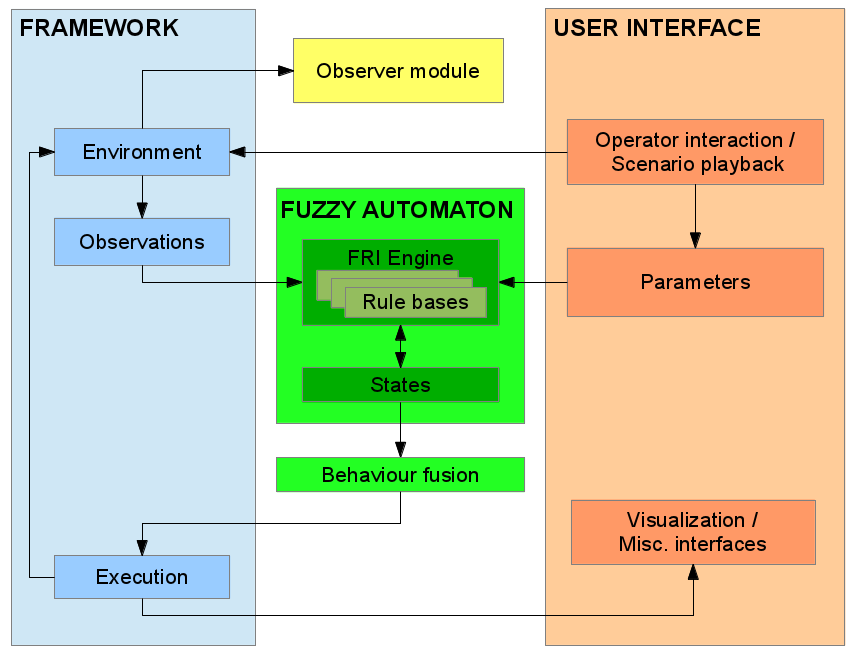
A screenshot of a possible simulation framework is shown in Fig. 6-5, where a room can be seen viewed from above, where the interactions take place. The humans are symbolized with squares, the blue square represents the owner of the dog, the magenta square represents a human unfamiliar (stranger) to the dog. The dog is represented by two circles, the large circle is the body of the dog, the smaller circle is the head of the dog, which is useful for visualizing the direction of the dog A thin green line on the dog’s body represents the tail of dog, which can change its length and also its angle (tail wagging). The color of the dog is dynamically changing showing the actual anxiety level of the dog. The room has a door where the human participants can leave or enter the room, the dog cannot go outside. Also a toy object is present (small blue circle, with a hole inside), which can be picked up and dropped by all the participants.
In the followings some example behaviours from the system and their definitions are presented.
The first example behaviour set is built upon two separate component behaviours, namely ‘DogExploresTheRoom’ and ‘DogGoesToDoor’. The ‘DogExploresTheRoom’ is an exploration dog activity, in which the dog ‘looks around’ in an unknown environment (see the track marked with white in Fig. 6-6). The ‘DogGoesToDoor’ is a simple dog activity, in which the dog goes to the door, and than stands (sits) in front of it (waiting for its owner to show up again). The definition of the related state-transition FRI rules of the fuzzy automaton acts as behaviour coordination in this example.
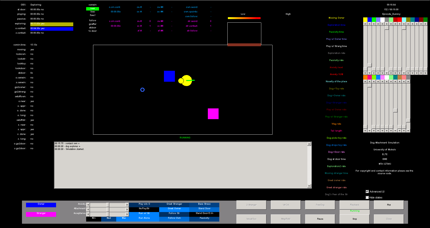
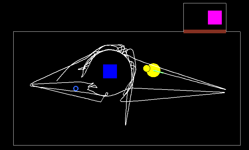
The states concerned are the following:
‘Hidden’ states, which have no direct task in controlling any of the above mentioned behaviours, but has an importance in the state-transition rule base: ‘Missing the owner mood of the Dog’ (DogMissTheOwner) and ‘Anxiety level of the Dog’ (DogAnxietyLevel).
‘Normal’ states, which have a direct task in controlling the corresponding ‘DogExploresTheRoom’ and ‘DogGoesToDoor’ behaviours: ‘Going to the door mood of the Dog’ (DogGoesToDoor) and ‘Room exploration mood of the Dog’ (DogExploresTheRoom).
As a possible rule base structure for the state-transitions of the fuzzy automaton, the following is defined (considering only the states and behaviours for this example):
State-transition rules related to the missing the owner mood (state) of the Dog:
If OwnerInTheRoom=False Then DogMissTheOwner=Increasing
If OwnerInTheRoom=True Then DogMissTheOwner=Decreasing
State-transition rules related to the anxiety level (state) of the Dog:
If OwnerToDogDistance=Small And Human2ToDogDistance=High Then DogAnxietyLevel=Decreasing
If OwnerToDogDistance=High And Human2ToDogDistance=LowThen DogAnxietyLevel=Increasing
State-transition rules related to the going to the door mood (state) of the Dog:
If OwnerInTheRoom=False And DogMissTheOwner=High Then DogGoesToDoor=High
If OwnerInTheRoom=True Then DogGoesToDoor=Low
State-transition rules related to the room exploration mood (state) of the Dog:
If DogAnxietyLevel=Low And OwnerStartsGame=False And ThePlaceIsUnknown=High Then DogExploresTheRoom=High
If ThePlaceIsUnknown=Low Then DogExploresTheRoom=Low
If DogAnxietyLevel=High Then DogExploresTheRoom=Low
The text in italic represent the linguistic terms (fuzzy sets) of the FRI rule base.
Also it should be noted that the rule base is sparse, containing the main state-transition FRI rules only.
A sample run of the example is introduced in Fig. 6-6 and in Fig. 6-7. At the beginning of the scene, the owner is in the room and the stranger is outside. The place is unknown for the dog (‘ThePlaceIsUnknown=High’ in the rule base). According to the above rule base, the dog starts to explore the room (see Fig. 6-6). After a little while the owner of the dog leaves the room, and then the stranger enters and stays inside (dashed white tracks in Fig. 6-7). As an effect of the changes (according to the above state-transition rule base), the anxiety level of the dog and the ‘Missing the owner’ state is increasing and as a result, the dog goes to and stays at the door (white track in Fig. 6-7), where its owner has left the room. See the state changes in Fig. 6-8.
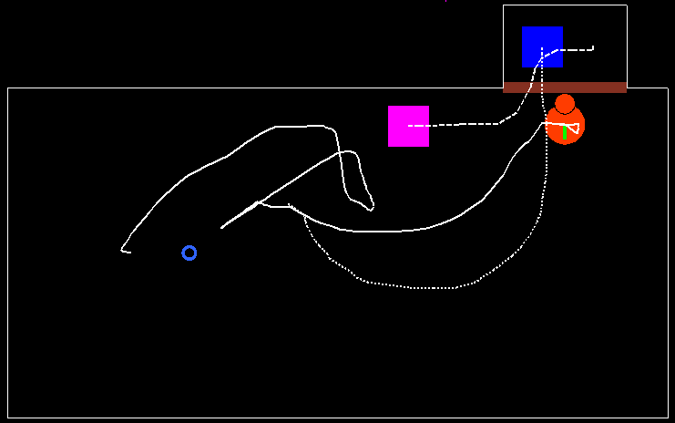
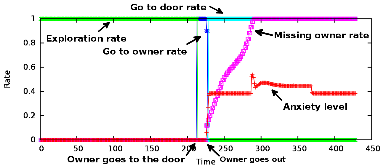
Fig. 68 shows the values of four state variables on a time scale (iteration number). Two immediate changes can be seen which are both caused by events related to the movement of the owner. First when the dog realizes that the owner is heading for the door (around the 200th iteration) the exploration rate drops rapidly and the rate of the ‘DogGoesToOwner’ behaviour component is high, till the owner finally leaves the room (around the 250th iteration). When the owner had left the room, the‘DogGoesToDoor’ behaviour component will be active, causing the value of the ‘Missing the owner’ state to increase. At the same time the anxiety level of the dog also increases with the leaving of the owner.
In the second example the ‘DogGoesToOwner’ behaviour will be presented in details from another point of view than the previous example. As its name suggests, this behaviour component is responsible for determining the need to go to the owner for the dog. The description of this behaviour component is more complex than the rule base in the previous example. The complete rule base for the ‘DogGoesToOwner’ behaviour is shown in REF _Ref364164389 \h , where the last column means the consequent part, all the other columns are antecedent dimensions (the ‘x’ value in the rule description means that the value of that antecedent is omitted while reasoning – does not have effect in the rule). The explanation of the terms used in the rule base is the following (‘observation’ in this case means that the value is gathered (measured) directly from the environment, ‘previous state’ means that the value was calculated in the previous iteration as a conclusion of a rule base):
dgtd – previous state – dog goes to door rate (zero-large) – see Fig. 6-12 for the corresponding fuzzy partition
dgto – previous state – dog goes to owner rate (zero-large) – see Fig. 6-12 for the corresponding fuzzy partition
oir – observation – owner is inside (true-false) – see Fig. 6-9 for the corresponding fuzzy partition
ddo – observation – distance between dog and owner (zero-large) – see Fig. 6-10 for the corresponding fuzzy partition
dgtt – previous state – dog goes to toy rate (zero-large) – see Fig. 6-9 for the corresponding fuzzy partition
dgro – previous state – dog greets owner rate (zero-large) – see Fig. 6-9 for the corresponding fuzzy partition
dpmo – previous state – dog’s playing mood rate with the owner (zero-large) – see Fig. 6-9 for the corresponding fuzzy partition
dpms – previous state – dog’s playing mood rate with the stranger (zero-large) – see Fig. 6-9 for the corresponding fuzzy partition
danl – previous state – dog’s anxiety level (zero-large) – see Fig. 6-11 for the corresponding fuzzy partition
ogo – observation – owner is going outside (true-false) – see Fig. 6-9 for the corresponding fuzzy partition
dgto (consequent) – next state – dog goes to owner rate (zero-large) (output)
|
# |
dgtd |
dgto |
oir |
ddo |
dgtt |
dgro |
dpmo |
dpms |
danl |
ogo |
dgto |
|
1 |
dgtdl |
x |
oirt |
x |
x |
x |
x |
x |
x |
x |
dgtoz |
|
2 |
dgtdz |
x |
oirt |
x |
dgttz |
dgrol |
x |
dpmsz |
x |
ogof |
dgtol |
|
3 |
dgtdz |
x |
oirt |
x |
dgttz |
x |
x |
dpmsz |
danll |
ogof |
dgtol |
|
4 |
dgtdz |
x |
oirt |
x |
dgttz |
x |
dpmol |
x |
x |
ogof |
dgtol |
|
5 |
dgtdz |
x |
oirt |
x |
x |
x |
x |
x |
x |
ogot |
dgtol |
|
6 |
dgtdz |
x |
oirt |
x |
x |
dgroz |
dpmoz |
x |
danlz |
ogof |
dgtoz |
|
7 |
x |
x |
oirf |
x |
x |
dgroz |
x |
x |
x |
ogof |
dgtoz |
|
8 |
dgtdz |
x |
x |
x |
dgtth |
dgroz |
x |
dpmsz |
x |
ogof |
dgtoz |
|
9 |
dgtdz |
x |
x |
x |
x |
dgroz |
x |
dpmsl |
x |
ogof |
dgtoz |
|
10 |
dgtdz |
dgtol |
oirt |
ddoz |
dgttz |
dgroz |
dpmoz |
dpmsz |
x |
ogof |
dgtoz |
|
11 |
dgtdz |
dgtol |
oirt |
ddol |
dgttz |
x |
x |
dpmsz |
x |
x |
dgtol |
The rules can be interpreted as the following textual description, in the corresponding order:
dog goes to door do not go to owner
dog should greet the owner go to owner
dog is nervous go to owner
dog's playing mood with owner is high go to owner
owner is going out of the room go to owner (follow the owner)
dog is calm and dog is not playing and not greeting do not go to owner
owner outside do not go to owner (can’t go to the owner)
dog is going to the toy do not go to owner
dog's playing mood with stranger is high do not go to owner
already going to owner and owner is near do not go to owner (arrived at the owner)
already going to owner and owner is far going to owner (keep on going)
The presented rule base is suitable to define a complex behaviour component with only eleven rules in spite of the relatively high antecedent dimension count (ten variables) thanks to the usage of FRI. In Fig. 6-9 through Fig. 6-12 the fuzzy partitions used for the various antecedents are presented. From top to bottom the curves in the mentioned figures show the membership functions, the scaling functions REF _Ref385687747 \r \h and the reconstructed membership functions (based on the scaling function). As it can be seen most of the fuzzy partitions are simple (six of the nine antecedents use the same simple fuzzy partition), consisting of only two triangular fuzzy sets with their cores at 0 and 1, and steepness of 1 on the right and the left side respectively. This is true also for the other rule bases in the model, most of the antecedent variables are defined by fuzzy partitions exactly like the one shown in Fig. 6-9.
Most of the behaviour components defined in the system are responsible for coordinating the movement (heading direction) of the dog, which must be aggregated by some kind of behaviour fusion. The simulation uses a simple weighted sum of the currently required behaviour components for determining the movement vector of the agent. Other behaviour components can be executed in parallel with movement related components. Also there are rule bases which are responsible for calculating the rate of behaviour components which are not directly executed, but instead their values are used by other rule bases as input values (in a hierarchical manner). E.g. the ‘DogGreetsOwner’ component is not executed directly, as shown in REF _Ref364164389 \h \* MERGEFORMAT . the consequent of ‘DogGreetsOwner’ is used as an input value in the rule base of the ‘DogGoesToOwner’ behaviour component, hence the actual output behaviour will be triggered by the activation of the ‘DogGoesToOwner’ behaviour component.
The model can be customized for different types of dogs. The system provides three factors for customization (‘Parameters’ in Fig. 6-4), which can be set in the interval [0,1]: ‘Anxiety’, ‘Acceptance’, and ‘Attachment’. The ‘Anxiety’ parameter defines the level of anxiety of the dog on a scale between calm and nervous, ‘Acceptance’ defines the level of the dog’s acceptance towards the stranger (between friendly and unfriendly), ‘Attachment’ defines the level of attachment of the dog to its owner (between weak and strong attachment). In fact these parameters are not directly used in the behaviour description rule bases. Secondary variables are calculated first based on the three parameters. Then these secondary parameters are used in the corresponding fuzzy rule bases. The three external parameters (‘Anxiety’, ‘Attachment’, ‘Acceptance’) mentioned earlier are used as antecedents in various rule bases, which have the task of determining the values of secondary parameters. These secondary parameters are then directly used as antecedents in the rule bases of the fuzzy automaton driving the simulation. These calculated secondary parameters are the following:
Play without the owner (when the owner is outside)
Do not play with the stranger (even when it could be possible)
Run in circles (caused by anxiety) when stranger is inside
Run in circles (caused by anxiety) when the dog is alone
Base rate of greeting the stranger
Base rate of greeting the owner
Base rate of following the stranger, when he/she is leaving the room
Base rate of greeting the owner, when he/she is leaving the room
Base rate of stress (anxiety)
Base rate of standing at the door
Base rate of standing at the door, even when the owner is inside
Base rate of passivity
This hierarchical strategy is useful for minimizing the input dimensions of the rule bases (one input variable is used instead of three input values in this case), hence fewer rules are required. The values of the secondary parameters are also calculated using fuzzy rule interpolation, each secondary parameter having its own rule base for determining the exact value based on the three input parameters. These are calculated at the time of initialization before starting the simulation, but can be also adjusted while the simulation is running, allowing the operator to switch between different types of dogs in real-time.
A distinct, but important part of the framework is the so called observer module (see Fig. 6-4), which has the task of evaluating the model (the correctness of the constructed rule bases) itself. The observer module only gets information from the environment (just what an outsider would see), no data about the inner states of the fuzzy automaton or behaviour weights are supplied to the observer. Based on these observations the observer module is able to determine what kind of activity is going on in the simulation. It can distinguish among ‘playing’, ‘exploring’, ‘standing at door’ and ‘passive’ states. If the dog is in contact (close the human and looking at the human) with the owner or the stranger, that is also measured and logged. Furthermore a special scoring system developed by ethologists used for evaluating the separation and reunion episodes (human leaves dog / human comes back) is also implemented in the observer module. Also the overall time spent in the various states along the different episodes is measured. A summary of the measurements and the scores is calculated at the end of the simulation, which can be directly used by ethologist experts to evaluate the simulated dog in the same manner as they would with real dogs.
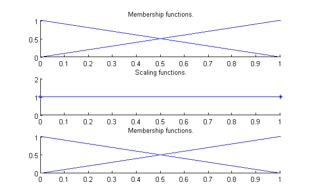
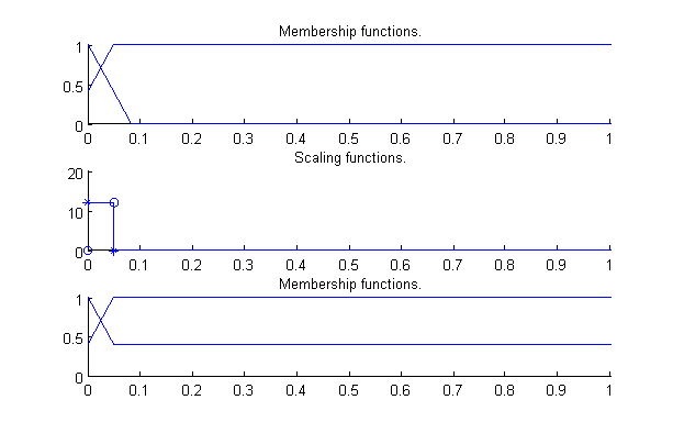
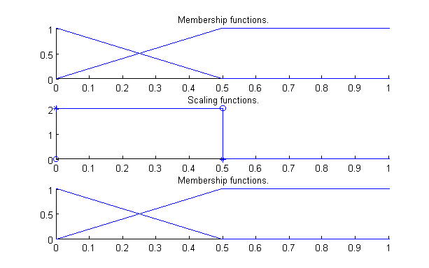
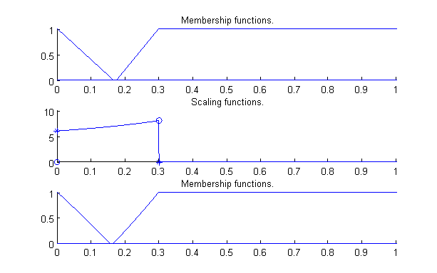
6.5. References for Fuzzy automaton for describing ethological functions
|
[1] |
D. Calisi, A. Censi, L. Iocchi és D. Nardi, „OpenRDK: a modular framework for robotic software development,” in Intelligent Robots and Systems, 2008. IROS 2008. IEEE/RSJ International Conference on, 2008. |
|
[2] | |
|
[3] | |
|
[4] |
„OpenRTM-aist robot middleware official web page,” [Online]. |
|
[5] |
N. Ando, S. Kurihara, G. Biggs, T. Sakamoto, H. Nakamoto és T. Kotoku, „Software deployment infrastructure for component based rt-systems,” Journal of Robotics and Mechatronics, %1. kötet23, %1. szám3, 2011. |
|
[6] |
N. Ando, T. Suehiro és T. Kotoku, „A software platform for component based rt-system development: Openrtm-aist,” in Simulation, Modeling, and Programming for Autonomous Robots, Springer, 2008. |
|
[7] |
N. Ando, T. Suehiro, K. Kitagaki, T. Kotoku és W.-K. Yoon, „RT-middleware: distributed component middleware for RT (robot technology),” in Intelligent Robots and Systems, 2005.(IROS 2005). 2005 IEEE/RSJ International Conference on, 2005. |
|
[8] | |
|
[9] |
M. Quigley, K. Conley, B. Gerkey, J. Faust, T. Foote, J. Leibs, R. Wheeler és A. Y. Ng, „ROS: an open-source Robot Operating System,” in ICRA workshop on open source software, 2009. |
|
[10] |
K. Saito, K. Kamiyama, T. Ohmae and T. Matsuda, "A microprocessor-controlled speed regulator with instantaneous speed estimation for motor drives," IEEE Trans. Ind. Electron., vol. 35, no. 1, pp. 95-99, Feb. 1988. |
|
[11] |
A. G. Filippov, "Application of the theory of differential equations with discontinuous right-hand sides to non-linear problems in autimatic control," in 1st IFA congress, 1960, pp. 923-925. |
|
[12] |
A. G. Filippov, "Differential equations with discontinuous right-hand side," Ann. Math Soc. Transl., vol. 42, pp. 199-231, 1964. |
|
[13] |
Van, Doren and Vance J., "Loop Tuning Fundamentals," Control Engineering. Red Business Information, July 1, 2003. |
|
[14] |
C. Chan, S. Hua and Z. Hong-Yue, "Application of fully decoupled parity equation in fault detection and identification of dcmotors," IEEE Trans. Ind. Electron., vol. 53, no. 4, pp. 1277-1284, June 2006. |
|
[15] |
F. Betin, A. Sivert, A. Yazidi and G.-A. Capolino, "Determination of scaling factors for fuzzy logic control using the sliding-mode approach: Application to control of a dc machine drive," IEEE Trans. Ind. Electron., vol. 54, no. 1, pp. 296-309, Feb. 2007. |
|
[16] |
J. Moreno, M. Ortuzar and J. Dixon, "Energy-management system for a hybrid electric vehicle, using ultracapacitors and neural networks," IEEE Trans. Ind. Electron., vol. 53, no. 2, pp. 614-623, Apr. 2006. |
|
[17] |
R.-E. Precup, S. Preitl and P. Korondi, "Fuzzy controllers with maximum sensitivity for servosystems," IEEE Trans. Ind. Electron., vol. 54, no. 3, pp. 1298-1310, Apr. 2007. |
|
[18] |
V. Utkin and K. Young, "Methods for constructing discountnuous planes in multidimensional variable structure systems," Automat. Remote Control, vol. 31, no. 10, pp. 1466-1470, Oct. 1978. |
|
[19] |
K. Abidi and A. Sabanovic, "Sliding-mode control for high precision motion of a piezostage," IEEE Trans. Ind. Electron., vol. 54, no. 1, pp. 629-637, Feb. 2007. |
|
[20] |
F.-J. Lin and P.-H. Shen, "Robust fuzzy neural network slidingmode control for two-axis motion control system," IEEE Trans. Ind. Electron., vol. 53, no. 4, pp. 1209-1225, June 2006. |
|
[21] |
C.-L. Hwang, L.-J. Chang and Y.-S. Yu, "Network-based fuzzy decentralized sliding-mode control for cat-like mobile robots," IEEE Trans. Ind. Electron., vol. 54, no. 1, pp. 574-585, Feb. 2007. |
|
[22] |
M. Boussak and K. Jarray, "A high-performance sensorless indirect stator flux orientation control of industion motor drive," IEEE Trans. Ind. Electron., vol. 53, no. 1, pp. 614-623, Feb. 2006. |
|
[23] |
D. C. Biles And P. A. Binding, „On Carath_Eodory's Conditions For The Initial Value Problem,” Proceedings Of The American Mathematical Society, %1. kötet125, %1. szám5, pp. 1371{1376 S 0002-9939(97)03942-7 , 1997. |
|
[24] |
Filippov, A.G., „Application of the Theory of Differential Equations with Discontinuous Right-hand Sides to Non-linear Problems in Automatic Control,” in 1st IFAC Congr., pp. 923-925, Moscow, 1960. |
|
[25] |
Filippov, A.G., „Differential Equations with Discontinuous Right-hand Side,” Ann. Math Soc. Transl., %1. kötet42, pp. 199-231, 1964. |
|
[26] |
Harashima, F.; Ueshiba, T.; Hashimoto H., „Sliding Mode Control for Robotic Manipulators",” in 2nd Eur. Conf. On Power Electronics, Proc., pp 251-256, Grenoble, 1987. |
|
[27] |
P. Korondi, L. Nagy, G. Németh, „Control of a Three Phase UPS Inverter with Unballanced and Nonlinear Load,” in EPE'91 4th European Conference on PowerElectronics, Proceedings vol. 3. pp. 3-180-184, Firenze, 1991. |
|
[28] |
P. Korondi, H. Hashimoto, „Park Vector Based Sliding Mode Control K.D.Young, Ü. Özgüner (editors) Variable Structure System, Robust and Nonlinear Control.ISBN: 1-85233-197-6,” Springer-Verlag, %1. kötet197, %1. szám6, 1999. |
|
[29] |
P.Korondi, H.Hashimoto, „Sliding Mode Design for Motion Control,” in Studies in Applied Electromagnetics and Mechanics, ISBN 90 5199 487 7, IOS Press 2000.8, %1. kötet16, 2000. |
|
[30] |
Satoshi Suzuki, Yaodong Pan, Katsuhisa Furuta, and Shoshiro Hatakeyama, „Invariant Sliding Sector for Variable Structure Control,” Asian Journal of Control, %1. kötet7, %1. szám2, pp. 124-134, 2005. |
|
[31] |
P. Korondi, J-X. Xu, H. Hashimoto, „Sector Sliding Mode Controller for Motion Control,” in 8th Conference on Power Electronics and Motion Control Vol. 5, pp.5-254-5-259. , 1998. |
|
[32] |
Xu JX, Lee TH, Wang M, „Design of variable structure controllers with continuous switching control,” INTERNATIONAL JOURNAL OF CONTROL, %1. kötet65, %1. szám3, pp. 409-431, 1996. |
|
[33] |
Utkin, V. I., „Variable Structure Control Optimization,” Springer-Verlag, 1992. |
|
[34] |
Young, K. D.; Kokotovič, P. V.; Utkin, V. I., „A Singular Perturbation Analysis of High-Gain Feedback Systems,” IEEE Trans. on Automatic Control, %1. kötet, összesen: %2AC-22, %1. szám6, pp. 931-938, 1977. |
|
[35] |
Furuta, K., „Sliding Mode Control of a Discretee System,” System Control Letters, %1. kötet14, pp. 145-152, 1990. |
|
[36] |
Drakunov, S. V.; Utkin, V. I., „Sliding Mode in Dynamics Systems,” International Journal of Control, %1. kötet55, pp. 1029-1037, 1992. |
|
[37] |
Young, K. D., „Controller Design for Manipulator using Theory of Variable Structure Systems,” IEEE Trans. on System, Man, and Cybernetics, %1. kötet, összesen: %2Vol SMC-8, pp. 101-109, 1978. |
|
[38] |
Hashimoto H.; Maruyama, K.; Harashima, F.: ", „Microprocessor Based Robot Manipulator Control with Sliding Mode",” IEEE Trans. On Industrial Electronics, %1. kötet34, %1. szám1, pp. 11-18, 1987. |
|
[39] |
Sabanovics, A.; Izosimov, D. B., „Application of Sliding Modes to Induction Motor,” IEEE Trans. On Industrial Appl., %1. kötet17, %1. szám1, p. 4149, 1981. |
|
[40] |
Vittek, J., Dodds, S. J., „Forced Dynamics Control of Electric Drive,” EDIS – Publishing Centre of Zilina University, ISBN 80-8070-087-7, Zilina, 2003. |
|
[41] |
Utkin, V.I.; „Sabanovic, A., „Sliding modes applications in power electronics and motion control systems,” Proceedings of the IEEE International Symposium Industrial Electronics, %1. kötetVolume of tutorials, pp. TU22 - TU31, 1999. |
|
[42] |
Sabanovic, A, „Sliding modes in power electronics and motion control systems,” in The 29th Annual Conference of the IEEE Industrial Electronics Society, IECON '03, Vol. 1, Page(s):997 - 1002, 2003. |
|
[43] |
Siew-Chong Tan; Lai, Y.M.; Tse, C.K., „An Evaluation of the Practicality of Sliding Mode Controllers in DC-DC Converters and Their General Design Issues,” in 37th IEEE Power Electronics Specialists Conference, PESC '06. Page(s):1 - 7, 2006. |
|
[44] |
Slotine,J.J., „Sliding Controller Design for Non-Linear Systems,” Int. Journal of Control, %1. kötet40, %1. szám2, pp. 421-434, 1984. |
|
[45] |
Sabanovic A., N. Sabanovic. K. Jezernik, K. Wada, „Chattering Free Sliding Modes,” The Third Worksop on Variable Structure Systems and Lyaponov Design , Napoly, Italy, 1994. |
|
[46] |
Korondi, H.Hashimoto, V.Utkin , „Direct Torsion Control of Flexible Shaft based on an Observer Based Discrete-time Sliding Mode,” IEEE Trans. on Industrial Electronics, %1. szám2, pp. 291-296, 1998. |
|
[47] |
Boiko, I.; Fridman, „ L Frequency Domain Input–Output Analysis of Sliding-Mode Observers,” IEEE Transactions on Automatic Control, %1. kötet51, %1. szám11, pp. 1798-1803, 2006. |
|
[48] |
Comanescu, M.; Xu, L., „Sliding-mode MRAS speed estimators for sensorless vector control of induction Machine,” IEEE Transactions on Industrial Electronics, %1. kötet53, %1. szám1, p. 146 – 153 , 2005. |
|
[49] |
Furuta.K. , Y.Pan, „Variable structure control with sliding sector,” Automatica, %1. kötet36, pp. 211-228, 2000. |
|
[50] |
Suzuki S, Pan Y, Furuta K, „VS-control with time-varying sliding sector - Design and application to pendulum,” ASIAN JOURNAL OF CONTROL, %1. kötet6, %1. szám3, pp. 307-316, 2004. |
|
[51] |
Korondi Péter, „Tensor Product Model Transformation-based Sliding Surface Design,” Acta Polytechnica Hungarica, %1. kötet3, %1. szám4, pp. 23-36, 2006. |
|
[52] |
Vadim Utkin, Hoon Lee, „The Chattering Analysis,” EPE-PEMC Proceedings 36, 2006. |
|
[53] |
Koshkouei, A.J.; Zinober, A.S.I., „Robust frequency shaping sliding mode control” Control Theory and Applications,” IEE Proceedings, %1. kötet147, %1. szám3, p. 312 – 320, 2000. |
|
[54] |
HASHIMOTO, H., and KONNO, Y., „‘Sliding surface design in thefrequency domain’, in ‘Variable Structure and Lyapunov control’,ZINOBER, A.S.I. (Ed.) (),,” Springer-Verlag, Berlin, pp. 75-84, 1994. |
|
[55] |
Koshkouei, A.J.; Zinober, A.S.I., „Adaptive backstepping control of nonlinear systems with unmatched uncertainty,” in Proceedings of the 39th IEEE Conference on Decision and Control, pp. 4765 – 4770, 2000 . |
|
[56] |
Kaynak, O.; Erbatur, K.; Ertugnrl, M., „The fusion of computationally intelligent methodologies and sliding-mode control-A survey,” IEEE Transactions on Industrial Electronics, %1. kötet48, %1. szám1, p. 4 – 17, 2001. |
|
[57] |
Lin, F.-J.; Shen, P., „H Robust Fuzzy Neural Network Sliding-Mode Control for Two,” Axis Motion Control System IEEE Transactions on Industrial Electronics, %1. kötet53, %1. szám4, p. 1209 – 1225 , 2006. |
Chapter 8. Models of Friction
8.1. Early Models of Friction
When one would like to examine the current achievements and theories, it worth to look back to the past and evaluate, how our predecessors interpreted the same problem. Below, a short summary is given concentrated only on the development of friction models, from the middle ages till the mid 20th century.
8.1.1. The first friction model
It is interesting, but probably not that surprising, that the first friction model came from Leonardo Da Vinci (1452-1519). Leonardo measured the force of friction between objects on both horizontal and inclined surfaces and he soon recognized the difference between rolling and sliding friction and the beneficial effect of lubricants.
As Figure 8-1 shows, Leonardo was curious of the influence of the apparent area. He wrote to his notebooks: “The friction made by the same weight will be of equal resistance at the beginning of its movement although the contact may be of different breadths and lengths.” The above observations are entirely in accord with the first two laws of friction. (see chapter 1.4.9)
Leonardo introduced first the coefficient of friction as the ratio of the force of friction and the normal load, however he assumed, that for smooth surfaces “every frictional body has a resistance of friction equal to one quarter of its weight.”
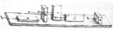
8.1.2. A more scientific approach
Robert Hook (1635-1703), inspired by the famous Stevin’s chariot [141] – a ship-like vehicle on wheels with masts, sails and other convenient riggings – discussed rolling friction and recognized two components: “…The first and chiefest, is the yielding, or opening of the floor, by the weight of the wheel so rolling and pressing; and the second, is the sticking and adhering of the parts of it to the wheel;…”
He further distinguished between the role of recoverable and non-recoverable deformation, and also discussed the question of sticking and adhesion.
Much of the scientific work of friction was initiated by Guillaume Amontons (1663-1705) of France. His experiments and interpretation of results were published in a classical paper presented to the Académie Royale in 1699.
The apparatus used by Amontons in his experiment is shown in Figure 8-2. The test specimens of AA and BB were loaded together by various springs denoted by CCC, while the force require to overcome friction and initiate sliding was measured on the spring balance D.
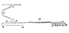
8.2. Friction phenomena
Friction is the tangential reaction force between two surfaces in contact. Physically these reaction forces are the results of many different mechanisms, which depend on contact geometry and topology, properties of the surface materials of the bodies, displacement and relative velocity of the bodies and presence of lubrication.
Contact surfaces are very irregular at microscopic level (see in Figure 8-3).
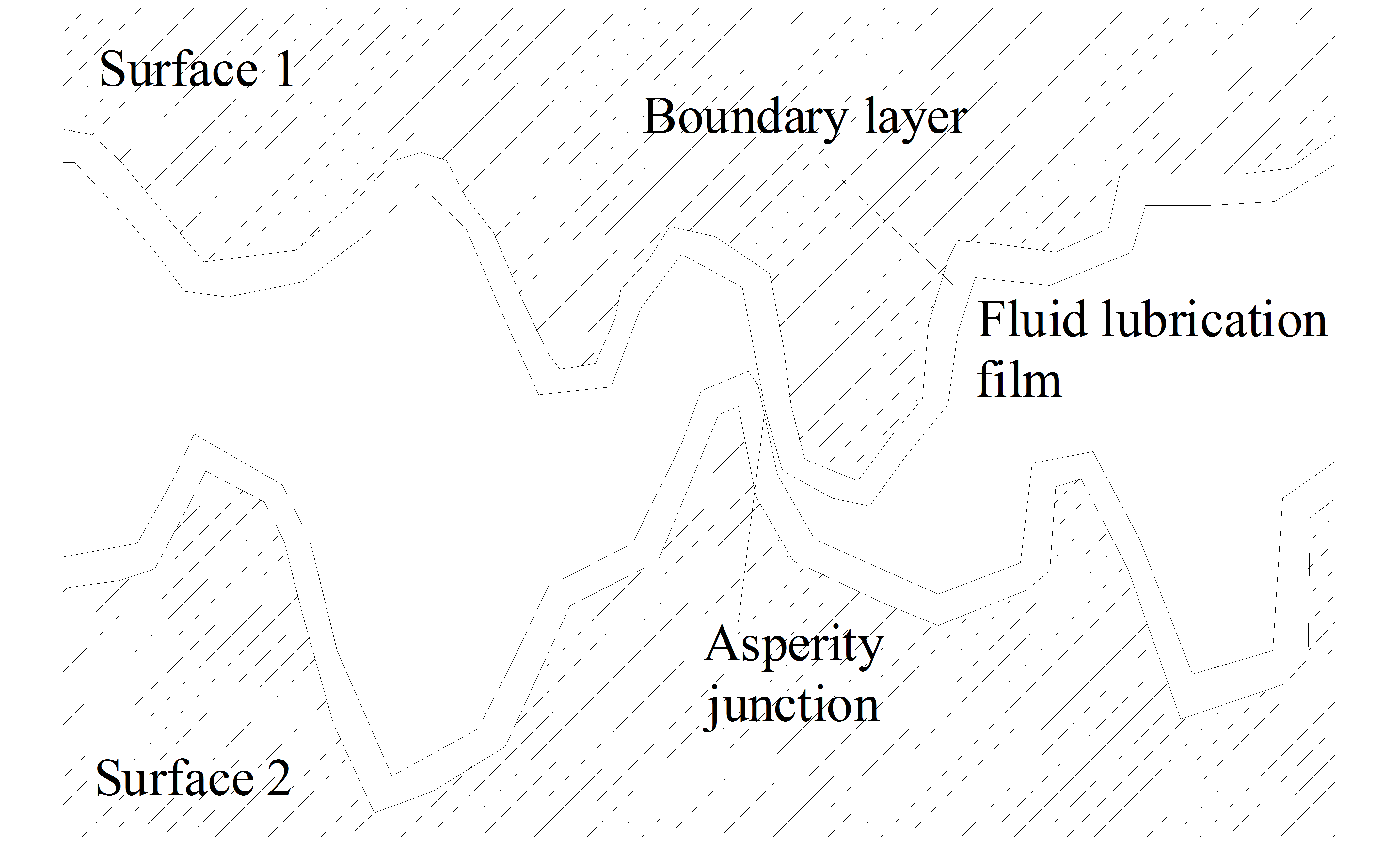
It can be visualized as two rigid bodies that make contact through elastic bristles (see in Figure 8-4).
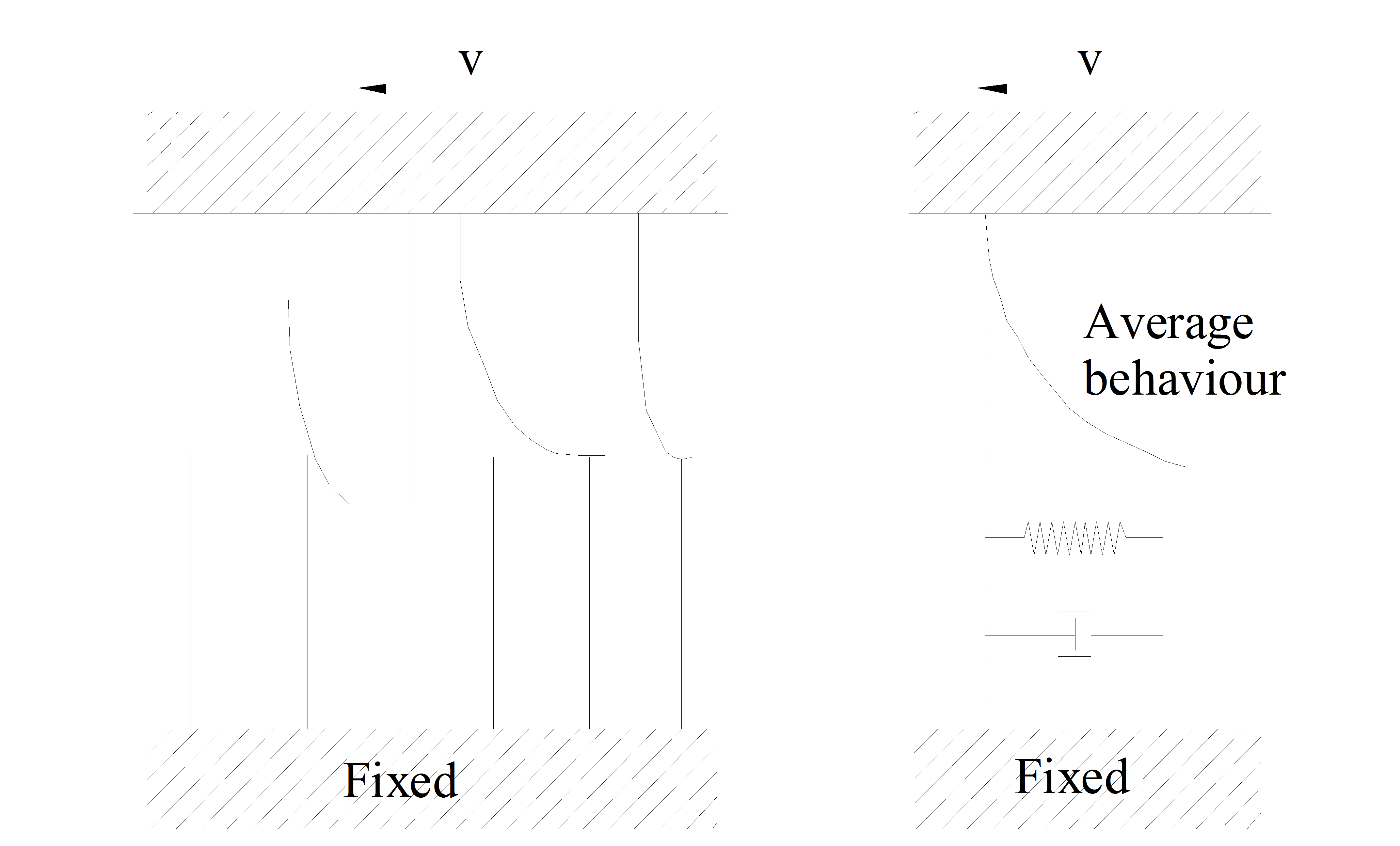
When tangential force is applied, the bristles will deflect like springs and dampers, giving raise to microscopic displacement (stick). If the displacement becomes too large, the bristles break (see in Figure 8-5).
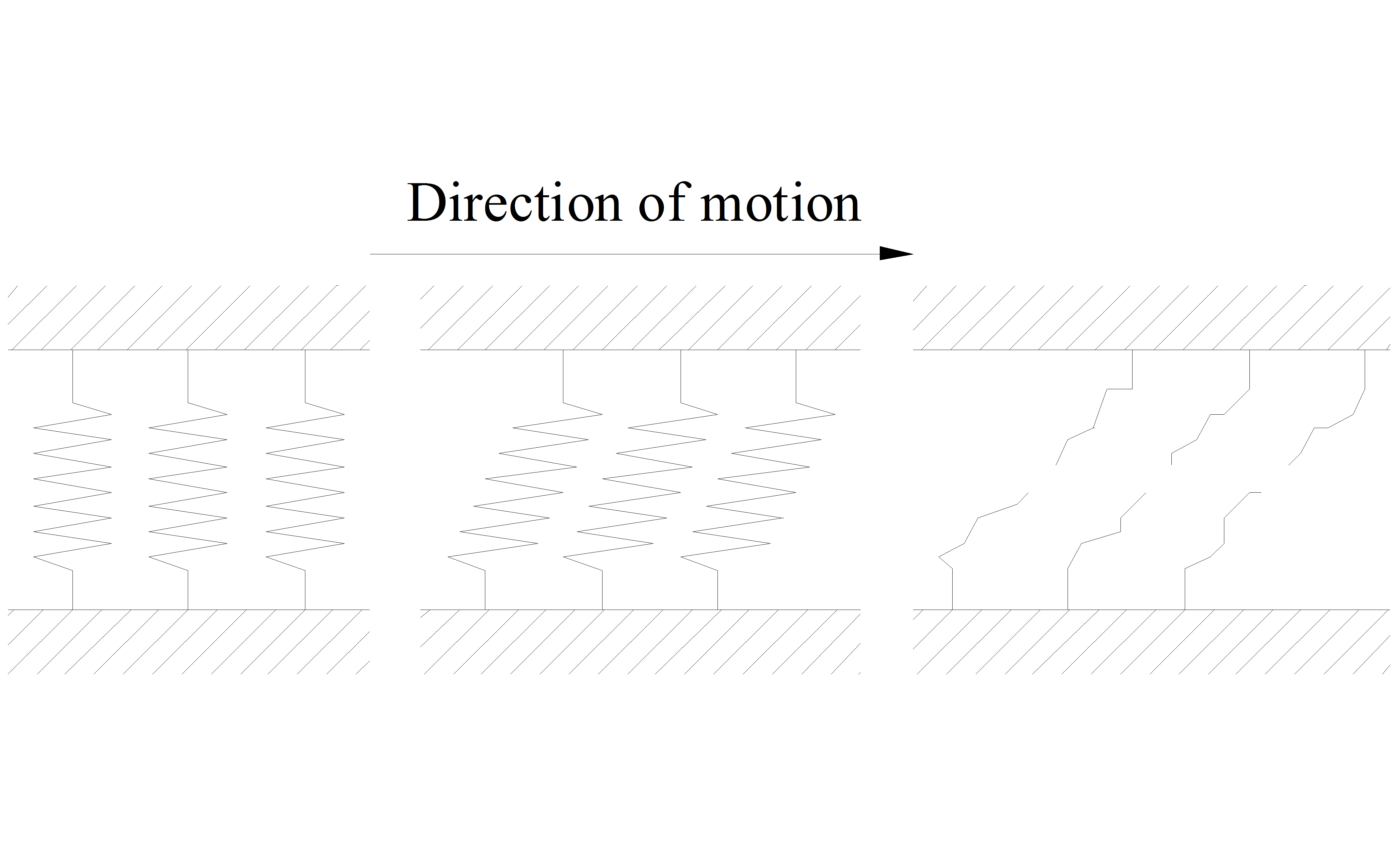
At this break-away displacement macroscopic sliding (slip) starts. The friction force where this occurs is called break-away force. The average deflection of the bristles corresponds to the internal state of the dynamic friction models. [10].
In dry sliding contacts between flat surfaces friction can be modeled as elastic and plastic deformation forces of microscopical asperities in contact. The asperities each carry a part fi of the normal load FN. If we assume plastic deformation of the asperities until the contact area of each junction has grown large enough to carry its part of the normal load, the contact area of each asperity junction is:
|
|
(8.1) |

where H is the hardness of the weakest material of the bodies in contact. The total contact area thus can be written
|
|
(8.2) |

This relation holds even with elastic junction area growth, provided that H is adjusted properly. For each asperity contact the tangential deformation is elastic until the applied shear pressure exceeds the shear strength τy of the surface materials, when it becomes plastic. In sliding the friction force thus is:
|
|
(8.3) |

and the friction coefficient:
|
|
(8.4) |

The friction coefficient is independent on the normal load or the velocity in this case. Consequently it is possible to manipulate friction characteristics by deploying surface films of suitable materials on the bodies in contact. [5].
As with many problems in the physical sciences, friction can be approached by using forces or by using energy. The best known model for friction that utilizes the force approach has been postulated by Bowden and Tabor. They suggested that surfaces adhere to form junctions and the friction force is directly related to the force needed to shear these junctions. The normal load FNis supported by the total contact area A of the deformed surfaces. If τjct is the shear strength of the adhesive junctions, then the frictional force:
|
|
(8.5) |
where PY is the yield pressure. Thus the coefficient of friction:
|
|
(8.6) |

Estimates of the friction coefficients from this expression have been reported as μ=0.2-0.3.
This model is based on the assumption of homogeneous and isotropic materials and uses a limited number of variables. Basic material characteristics tend to be neglected in most available model of friction. Microstructural information which significantly influences material behaviour is generally omitted.
Some plastic deformations always occur near the surfaces of sliding materials. Therefore plastic deformation and associated parameters such as microstructure as mentioned before are important parameters in setting up a more realistic friction model. P. Heilman and D. A. Rigney have presented an energy based model of friction. It is assumed that the frictional work is approximately equal to the plastic work done, or:
|
|
(8.7) |
where τ(γ) is the shear stress, γ is the shear strain and V is the deformed volume near to the surface. This approach is applicable for metals and for some polymers and ceramics, which can deform plastically under compressive loading.
In dry rolling contact, friction is the result of a non-symmetric pressure distribution in the contact. The pressure distribution is caused by elastic hysteresis in either of the bodies, or local sliding in the contact. For rolling friction the friction coefficient is proportional to the normal load as
|
|
(8.8) |
The elastoplastic characteristics of dry friction can be described by hysteresis theory.
Other physical mechanisms appear when lubrication is added to the contact. For low velocities, the lubricant acts as a surface film, where the shear strength determines the friction. At higher velocities at low pressures a fluid layer of lubricant is built up in the surface due to hydrodynamic effects. Friction is then determined by shear forces in the fluid layer. These shear forces depend on the viscous character of the lubricant, as well as the shear velocity distribution in the fluid film. Approximate expressions for the friction coefficient exist for a number of contact geometries and fluids. At high velocities and pressures the lubricant layer is built up by elastohydrodynamic effects. In these contacts the lubricant is transformed into an amorphous solid phase due to the high pressure. The shear forces of this solid phase turn out to be practically independent of the shear velocity. The shear strength of a solid lubricant film at low velocities is generally higher than the shear forces of the corresponding fluid film built up at higher velocities. As a result the friction coefficient in lubricated systems normally decreases when the velocity increases from zero. When the thickness of the film is large enough to completely separate the bodies in contact, the friction coefficient may increase with velocity as hydrodynamic effects become significant. This is called the Stribeck effect.
Film thickness is a vital parameter in lubricated friction. The mechanisms underlying the construction of the fluid film includes dynamics, thus suggesting a dynamic friction model. Contamination is another factor that adds complication. The presence of small particles of different materials between the surfaces give rise to additional forces that strongly depend on the size and material properties of the contaminants.
This short expose of some friction mechanisms illustrate the difficulty in modeling friction. There are many different mechanisms. To construct a general friction model from physical first principles is simply not possible. Approximate models exist for certain configurations. What we look for instead is a general friction model for control applications, including friction phenomena observed in those systems.
8.2.1. Friction - General observations
Talking about friction in general, we can summarize the basic, well-known properties in five points according to [111].
1.) In any situation where the resultant of the tangential forces is smaller than some force parameter specific to that particular situation, the friction force will be equal and opposite to the resultant of the applied forces and no tangential motion will occur.
2.) When tangential motion occurs, the friction force always acts in a direction opposite to that of the relative velocity of the surfaces.
3.) The friction force Ff is proportional to the normal force F. This relationship enables us to define the coefficient of friction :
|
F |
(8.9) |

Alternatively this law can be expressed in terms of a constant angle of repose or frictional angle , defined by:
|
tan = |
(8.10) |
It may readily be shown that is the angle of an inclined plane such, that any object, whatever its weight placed on the plane will remain stationary, but that if the angle is increased by any amount whatever, the object will slide down.
4.) The friction is independent the apparent area of contact Aa. Thus, large and small objects have the same coefficients of friction.
5.) The friction force is independent of the sliding velocity v. This implies that force required to initiate sliding will be the same as the force to maintain sliding at any specified velocity.
These frictional properties are widely used in the everyday life and often in the engineering practice. Despite, unfortunately, we can say they are simply and solely good approximations. The research of friction is going on, and tribology still contains many uncovered areas. What we can be already sure about is that the real picture is far more complex and many times surprisingly different from the given points above.
8.2.2. Origin of friction
The model described above dates back to the 18th century and still with us since the scientific achievements of Amontons and Coulomb. Thanks to the technological evolution the 20th century brought to life many new tools and methods backing up tribological researches and made possible to reconsider the interpretation of friction.
The Coulomb type model suffers from two great mistakes. On one hand the whole model lays basically on the roughness theory and claims that friction is based almost solely on surface roughness. The reason for this is simple. By that time special equipment and supplementary knowledge were missing to find out the connection between friction and adhesion. On the other hand in this way this model also fails to demonstrate convincing the dissipative nature of friction.
Although there were theories pointing towards the right direction [140], we can say that the real breakthrough happened during World War II, in 1943, in Australia. It was the series of experiments carried out Bowden and Tabor [24], which provided experimental evidence for earlier adhesion theories, and which gave a chance at last to explain frictional losses.
They studied the behavior of concentrated contacts – a sphere in contact with a flat [23], [24], [25]. As the surfaces were “smooth” they modeled the noncomformal contact of a single asperity so that the geometric area became a fair approximation of the real area. They used metal indium what is not only known as a very soft material (its hardness is about one quarter of the hardness of lead) but is also relatively inert, thus, the effect of oxide films is negligible.
They made three important observations.
First, the area of geometric contact was proportional to the load. The deformation was clearly plastic. This at once indicated that for extended surfaces each asperity deformed plastically under the load that it born, thus, the total area of contact was proportional to the total load.
The second was that the indium actually stuck with the other surface and a small, finite normal force was required to pull it off. Clearly strong interfacial bonds were formed. This phenomenon referred to adhesion between the two contacting surfaces.
The third observation was that in sliding there was plastic flow as the indium sheared away in its adhered region. When the system was inverted, and a hard sphere slid over indium they observed an additional resistance to sliding due to the work of plastically grooving the indium surface.
They experienced similar results with other material pairs. Extending the results of these experiments they attributed the friction to two factors [24], [25]. Which later works of Rabinowicz added two more to [111].
Friction is due to four main factors:
The adhesion of one surface to the other.
Plowing of the softer surface by asperities on the harder.
Roughness of the surfaces.
Electrical components.
In the previous chapters we took a look at to the origin and cause of friction as well as its forms of appearance. Below, we try to summarize the different approaches used for modeling this phenomenon.
8.3. Simple elements
Static models are mostly simple mathematical representations of certain frictional behaviors. They do not deal with friction as a complex process, only with some of its sub processes, such as frictional force at rest i.e. static friction, friction as a function of steady-state velocity, etc.
8.3.1. Coulomb friction
The easiest and probably the most well known model is the so-called Coulomb friction model. Though it greatly over simplifies the frictional phenomena it is widely used in the engineering world, when dynamic effects are not concerned. Also, the Coulomb model is a common piece of all more developed models. The Coulomb friction force Fc is a force of constant magnitude, acting in the direction opposite to motion:
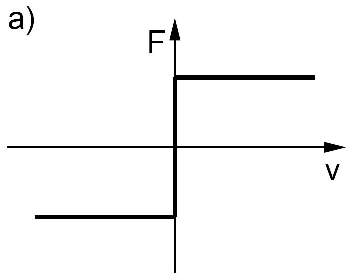
When:
|
|
(8.11) |

|
|
(8.12) |

Where FN is the force pressing surfaces together and μ is the frictional factor. μ is determined by measurements under certain conditions. One of the biggest problems of the Coulomb model is, that it cannot handle the environment of zero velocity, hence the properties of motion at starting or zero velocity crossing, i.e. static and rising static friction. To apply the model for those cases a μ0 factor has been introduced. In case of starting the motion it replaces μ in Equation (8.12) until the process arrives to steady state. The values of μ and μ0 can be found in any major physics or engineering tabulations for different material pairs in both dry and lubricated conditions. The first tabulations of those kinds date back to the beginning of 18th century. Note, that though this is the simplest and fastest way to calculate the frictional force, this method can suffer from the error up to 20%.
8.3.2. Viscous friction
The viscous friction element models the friction force as a force proportional to the sliding velocity:
When:
|
|
(8.13) |

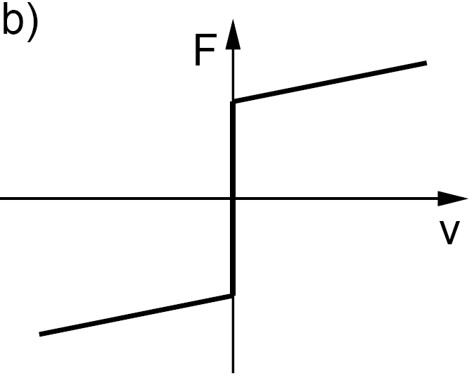
8.3.3. Static friction
Static friction is a force of constraint:
When

|
|
(8.14) |
where Fs is the static friction force, an additional upload on Fc, the Coulomb friction force.
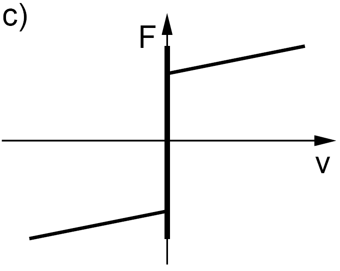
8.3.4. Stribeck effect
The Stribeck curve is a more advanced model of friction as a function of velocity. Although it is still valid only in steady state, it includes the model of Coulomb and viscous friction as built-in elements.
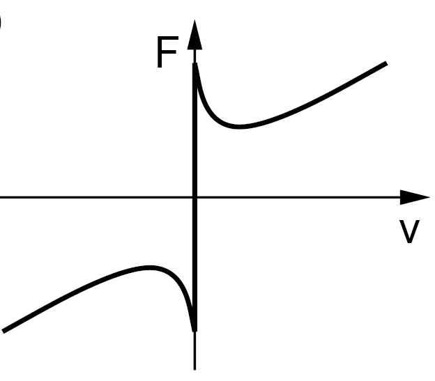
8.3.5. Presliding displacement
The presliding displacement was studied and modeled first by Dahl [40]. Recalling xxx he gives:
|
|
(8.15) |

where Ff(x) is the friction force as the function of presliding displacement, kt is the stiffness of the material and x is the displacement. kt is a material property, but can be calculated using Equation (8.15) such a way, that x is in the range of 1-50 [μm].
8.3.6. Rising static friction and dwell time
There are several models available describing this phenomenon. The empirical model of Kato [85] is:
|
|
(8.16) |
where  is the ultimate static friction, i.e. the magnitude of static friction after a long time of rest, FC is the Coulomb friction at the moment of arrival to stuck, and m are empirical parameters in the range of 0.04 to 0.64 and 0.36 to 0.67 respectively. Small means long rise time and thus resists thick slip. Examining non-conformal contacts Amstrong-Hélouvry finds = 1.66 and m = 0.65 [6].
Another model presented by Amstrong-Hélouvry [6] eliminates the use of FC as the starting point of the static friction rise. Thus the model has one fewer parameter than that of Equation (8.16).
|
|
(8.17) |

where  is the level of static friction at the beginning of the nth interval of slip, i.e. breakaway,
  is the level of static friction at the end of previous interval of slip,
  is the ultimate static friction, is an empirical parameter. Note that will be different in physical dimension from that of Equation (8.16).
8.3.7. Frictional memory
Frictional memory is modeled simply as a time lag:
|
|
(8.18) |
where Ff(t) is the instantaneous friction force, Fvel() is friction as a function of steady state velocity and t is the lag parameter. Measuring frictional time lag, Hess and Soom [75] find them in the range of 3 to 9 ms depending on the load and lubrication. They also show that the lag increasing with increasing lubricant viscosity and increasing contact load. However, it appears to be independent from oscillation frequency.
8.4. Complex models
Complex models are mostly built upon the simple model elements with additional features, which can handle dynamic behavior. Yet the science of tribology is still far from having a complete picture on how friction works in all extent, therefore these models are mostly based on empirical experiences, rather than deep scientific background.
8.4.1. Steady state models
8.4.1.1. Stribeck curve
The model below was employed by Hess and Soom [75].
|
|
(8.19) |
where the Coulomb, viscous and static friction is denoted by FC, Fv and Fs respectively. vs is the characteristic velocity of the Stribeck curve. Hess and Soom reported systematic dependence of Fv and vs on lubricant and loading parameters.
Another proposal for modeling the Stribeck effect is a linearized exponential equation of Bo and Pavelescu [21]. The viscous friction term was added by Armstrong-Hélouvry [9].
|
|
(8.20) |
where δ is an additional empirical parameter. In the literature surveyed by Bo and Pavelescu [21] they find the range of δ from 0.5 to 1. Armstrong-Hélouvry [6], [8] employs δ = 2 and Fuller [57] suggest δ = very large for systems with effective boundary lubricants. Applying δ = 2 the exponential model, Equation (8.20) becomes Gaussian model, which is nearly equivalent of the Lorentzian model of Equation (8.15).
8.4.1.2. Tustin model
Another simple representation of the Stribeck curve is the Tustin model [144]. The model captures the basic frictional phenomenon and simply superposes them on one another. The three features are the Coulomb friction FC, the static friction Fs with the downward bend of the negative viscous effect determined by α and the viscous friction Fv.
|
|
(8.21) |
Linearizing the Tustin model we get:
|
|
(8.22) |
This model although a linear one, leads to a precision of approximated friction only up to 85% in the region where the velocity comparable to its square root. In other cases where the system velocity is not so very low, another model should be used.
8.4.2. Dynamic models
8.4.2.1. Seven-parameters friction model
A popular approach is simply sewing together the already existing model elements. This is how the seven-parameters model works. Each of the seven parameters of the model represents a different friction phenomenon as presented in Table 8.2. They value principally depends upon the mechanism and the lubrication conditions, but typical values may be offered based on the works of [6], [27], [57], [75], [85], [105].
The friction is given by:
Not sliding (presliding displacement)
|
|
(8.23) |

Sliding (Coulomb + viscous + Stribeck curve friction with frictional memory)
|
|
(8.24) |
Rising static friction (frictional level at breakaway):
|
|
(8.25) |
Where:
|
Ff() |
is the instantaneous friction force |
|
FC |
(*) is the Coulomb friction force |
|
Fv |
(*) is the viscous friction force |
|
Fs |
is the magnitude of the Stribeck friction (frictional force at breakaway is FC+Fs) |
|
Fsa |
is the magnitude of the Stribeck friction at the end of the previous sliding period |
|
Fs |
(*) is the magnitude of Stribeck friction after a long time at rest (with a slow application of force) |
|
kt |
(*) is the tangential stiffness of the static contact |
|
vs |
(*) is the characteristic velocity of Stribeck friction |
|
L |
(*) is the time constant of frictional memory |
|
(*) is the temporal parameter of the rising static friction | |
|
t2 |
is the dwell time, time at zero velocity |
|
(*) |
marks friction model parameters, other variables are state variables |
|
Parameter range |
Parameter depends upon | |
|
FC |
0.001 0.1FN |
Lubricant viscosity, contact geometry and loading |
|
Fv |
0 very large |
Lubricant viscosity, contact geometry and loading |
|
Fs |
0 0.1FN |
Boundary lubrication, FC |
|
kt |
1/x(FC+Fs) x1 50 [m] |
Material properties and surface finish |
|
vs |
0.00001 0.1 [m/s] |
Contact geometry and loading |
|
L |
1 50 [ms] |
Lubricant viscosity, contact geometry and loading |
|
0 200 [s] |
Boundary lubrication |
|
Friction model |
Predicted/observed behavior |
|
Viscous |
Stability at all velocities and at velocity reversals |
|
Coulomb |
No stick-slip for PD control No hunting for PID control |
|
Static + Coulomb + Viscous |
Predicts stick-slip for certain initial conditions under PD control Predicts hunting under PID control |
|
Stribeck |
Needed to correctly predict initial conditions leading to stick-slip |
|
Rising static friction |
Needed to correctly predict interaction of velocity and stick-slip amplitude |
|
Frictional memory |
Needed to correctly predict interaction of stiffness and stick-slip amplitude |
|
Presliding displacement |
Needed to correctly predict small displacements while sticking (including velocity reversals) |
Parameter identification. The parameters, which represent a non-linear relationship with the friction force, cannot be identified by using linear methods. Kim et al proposes a possible non-linear identification method for the seven parameter model, the Accelerated Evolutionary Programming (AEP) [88] and gives the description as outlined below. AEP is a stochastic optimization technique for finding the extrema of an arbitrary function. A simple optimization problem can be stated as: determine the values of the ordered set of n parameters
|
|
(8.26) |
which minimize/maximize the cost function f(z). AEP is a genetic algorithm type method, working with parent/child interactions to converge to the best solution. It uses two variation operators. One of them, the direction operator determines the direction of the search according to the fitness score. The other one is a zero-mean Gaussian operator, used a perturbation added to a parent in order to generate an offspring. AEP also uses a further “age” variable to enhance the diversity of the search and to prevent individuals to remain in the local minima. The Gaussian operator is incorporated with both the direction operator and the variable age. Unlike another genetic methods, AEP generates only one child from its parent. New parents then are selected in one-to-one competition between parent and its child. An offspring is selected if the child wins in the competition with its parent. AEP incorporates the direction of evolution and the age concept into the vector to be optimized in order to increase the convergence speed without loosing the diversity. Thus it brings Equation (8.26) into the form of
|
|
(8.27) |

where  for all
 is the evolving direction of the jth parameter
  in
in  the ith vector, and agei denotes the duration of the life in an integer type in the ith vector. The following two rules are applied for perturbing the parents to generate their offspring.
Rule 1
When  ,
,
then  ,
,

or else  ,
,
|
|
(8.28) |
Rule 2
When  ,
,
then  ,
,
or else  ,
,
,
|
|
(8.29) |
where  denotes the jth parameter in the ith vector among Np vectors at the kth generation,
  denotes the evolving direction of
  ,
,  is a realization of a Gaussian-distributed random variable, which is polarized in the direction of
  , and i, i = 1, 2 are positive constants. Rule 1 indicates that if the performance of a newly generated child is better, then the search will continue towards the promising direction, by setting the direction value and generating a random number in the respective positive or negative region. Otherwise the parent will be kept, by increasing the age value. As Rule 2 “else” part shows, in the latter case the standard deviation of the Gaussian-distributed random variable is getting larger in each step, since the age is included in the product. It also makes more probable that the algorithm doesn’t stuck in the local minima but tends to find the global one.
The procedure of applying the AEP is as follows:
1.) Initialization. Generate an initial population of Np trial solutions with a uniform distribution within the given domain for the ith individual vector.
|
|
(8.30) |
where  és
és  ,
,  are randomly initialized and agei is initially set to 1.
2.) Evaluation. Evaluate the fitness of each parent solution by the given cost function f(zi).
3.) Mutation. For each of the Np parents zi, generate a child by using Rules 1 and 2 successively.
4.) Evaluation. Evaluate the fitness of each new offspring.
5.) Selection by one-to-one comparison. If the newly generated child is better than its parent, then select the child and discard the parent, else vice versa. New parents are composed of Np vectors selected among 2Np vectors by one-to-one comparison. The new Np parents are sorted by fitness score.
6.) Termination check. Proceed to step 3 unless available execution time is exhausted or acceptable solution has been discovered.
The most obvious way for parameter identification is to run parallel the experiment and AEP using the same input value. Parameters are identified, when the difference between the real and calculated output values diminish or fall into the previously defined error range. Input value can be position or velocity depending on the used sensor.
For the seven parameter model, first we need to know the input v or (dx/dt) and the state variables t2 and Fs,a. For this let us define a new state variable s, which indicates, whether the system is in stick or slip.
|
|
(8.31) |


where vcritical is specified by the resolution of the velocity/position sensor built into the real system. Depending on the change of the value of s, t2 and Fs,a are obtained as followed.
When s changes from
|
0 to 0: |
t2 t2 + Ts |
|
0 to 1: |
compute Fs,b |
|
1 to 0: |
Fs,a and t2 0 |
|
1 to 1: |
no operation |
where Ts is the sampling time.
Let a vector z denote the set of unknown parameters of Equation (8.24).
|
|
(8.32) |
where all the parameters are positive. The mismatched displacement error between the plant output and the identification output is
|
|
(8.33) |
where  denotes the estimate of z, x(z,ti) is a displacement of the plant, x(
 ,ti) is a displacement of the identification model at the sample time ti, and Ns is the total number of sample data. Consider the cost function of the squared errors is given by:
|
|
(8.34) |
Then the parameter identification problem can be posed as an optimization problem as follows:
|
|
(8.35) |

8.4.2.2. State variable friction model
Research in dynamic friction modeling of rocks in boundary lubrication carried out by geophysicist led to the born of the state variable friction model. [6], [16]. For constant normal stress, the general form including n state variables iis given by
Coming from this representation, a sudden change in velocity does not cause a change in but it does affect its time derivative. For a single state variable Ruina proposes the following frictional law [16]
|
|
(8.38) |
|
|
(8.39) |
Where is the scalar state variable, L is the characteristic sliding length controlling the evolution of . The pair (v0/f0) corresponds to any convenient point on the steady-state friction-velocity curve. The steady state curve is given by:
|
|
(8.40) |
and the steady state variable can be related to the mean lifetime of an asperity junction.
Limitations. Unfortunately the model structure itself imposes a limitation on the use of the state variable model. At standstill, the value of v/v0 in Equation (8.40) becomes zero, which gives infinitive friction force due to the result in the logarithmic function (ln 0 = ). In simulations normally it causes a problem in the integrator. A good approach to avoid it is to include a switch, which for zero velocity gives a finite friction value. However since  , it means that in the environment of very small velocities the value of the logarithmic function and thus the friction force changes very fast, resulting a strong dependence of error on the selected environment size. Hence for low velocities this model is not adequate.
Parameter identification. Dupont et al gives a detailed description on the measuring apparatus used for their experiment [49]. In principle any other methods can be used, thus we are not going into details of the original set up. The first step to identify the parameters of Equation (8.38) and Equation (8.39), one must draw the steady state velocity – friction curve (or Stribeck-curve) of the respective system. The change of velocity results a change in the system as well. This can be used to compute the values of A and B on the following way. The system’s response given to a velocity step imposed at time t0, where the pair (v1, f1) corresponds to the initial steady state, the pair (v2, f2) describes to the steady state reached after the step response, while fmax denotes the maximum friction force reached during the transient. The parameters A and B then calculated as:

The exponential decay of the state variable following a velocity step is given as
|
|
(8.43) |
The characteristic sliding length L can be computed from a least squares fit of the exponential to the data immediately following the velocity step.
Table 8.4 shows some state variable model parameter values calculated by Dupont et al. The used lubricants are as follows. The used lubricants are paraffin oil with maximum Saybolt viscosity of 158 and a commercial boundary lubricant paste. Test samples were made of heat-treated and oil quenched tool steel, with Rockwell hardness of 59 C.
|
Parameter |
Dry |
Paraffin Oil |
Boundary Lubricant |
|
A 103 |
2.8 0.5 |
0.0* |
1.1 0.1 |
|
B 103 |
9.4 1.1 |
11.1 2.5 |
4.0 0.4 |
|
L [m] |
64.7 14.3 |
22.4 4.3 |
19.2 1.4 |
The magnitude was less then noise level of the measurement.
8.4.2.3. Karnopp friction model
In some model representations friction may be a discontinuous function of the steady-state velocity. In case of integrating discontinuous ordinary differential equations it may cause a problem, though with embedded switching functions this problem is still manageable. In addition, the integrator also has to bear with the ability to locate the point of discontinuity within the given interval. Variable-step-size variable-order methods are appropriate for this purpose and they are built in elements in all commercially available simulation software. However in the physical representation of a controller in the majority of cases we have to use fixed-step-size methods as the sampling time is fixed.
The Karnopp [84] model solves this problem by introducing a pseudo velocity and a small neighborhood of zero velocity ±DV in which the speed is set to zero. The pseudo velocity, p(t) which in the original material is referred as momentum, is integrated on the standard way.
|
|
(8.44) |
where Fa is the force acting on the system, while Fm is the modeled friction force. The velocity of the system is set according to Equation (8.45), where M is the system mass.
|
|
(8.45) |

The friction law is given as:
|
|
(8.46) |

This includes the Coulomb, static and viscous terms (FC, Fs, Fv respectively) but can be upgraded with any other convenient curves (e.g. Stribeck curve).
8.4.2.4. LuGre model
Unlike the seven parameter model, the LuGre model is an integrated dynamic friction model. In some sources it is also referred as “integrated dynamic model”. The name comes from the abbreviation of the Lund Institute of Technology and INPG Grenoble, the two universities hosting the cooperating scientists. The LuGre model is based on the elasticity in the contact [33]. The variable z(t) represents the friction state and can be interpreted as the mean deflection of the junctions between the two sliding surfaces. The instantaneous friction Ff is given by
|
|
(8.47) |
where σ0 describes the stiffness for a spring-like behavior for small displacements, and σ1 gives the negative viscous friction term. The state variable is updated according to:
|
|
(8.48) |
where
|
|
(8.49) |
Fc, Fs and Fv represents the Coulomb, Stribeck and static friction respectively. For some special cases, an additional element Fg can be added to the sum, representing the effect of gravity (e.g. in case of dealing with a vertical machining axis) or amplifier offsets. The steady-state friction is as follows:
|
|
(8.50) |
The advantage of this model, is that besides it is valid in both rotational and linear coordinates, it describes the phenomena for normally flat surfaces as well as for rolling bearings element
Parameter identification. An identification method is presented in [2] based on the general methods used for linear dynamic systems. Note that the method includes Fg contrary to Equation (8.47)-(8.49). The parameters Fs and σ0 are easily deduced from the Dahl’s curve.
The assumption  implies Fs=F. Furthermore, if
  , then
  and
and  . Combining (8.50) with these assumptions leads to
|
|
(8.51) |
Using Euler’s approximation for time derivatives, a linear regression results
|
|
(8.52) |
The authors of [1] concluded that these algorithms turned to be sensitive to position measurement noise, thus they propose to use interferometers instead of inductive sensors to eliminate the bias on  .
.
8.4.2.5. Modified Dahl model
The original Dahl model [40], [20] predicts a frictional lag between the velocity reversals and leads to hysteresis loops. It does not contain however the Stribeck effect. To overcome on this deficiency Canudas et al proposed to transform the Dahl model into a second order linear space invariant model, which emulates the Stribeck friction by producing an overshoot in the response of friction forces. However, doing so, they also eliminated the dissipative properties of the first order model. The modified Dahl model is a first order model redesigned by Canudas et al and this time combining the Stribeck phenomenon without increasing the system state dimension.
The friction force represented by Ff is described by

where ε is a time constant proportional to 1/vsimilarly to the original Dahl model, z is a state variable should be interpreted as an “internal” friction state, vs is the characteristic velocity of the Stribeck curve, while α1, α2 and α3 are positive constants representing the Coulomb, Stribeck and viscous friction terms respectively.
The steady state friction is given by:
|
|
(8.56) |
8.4.2.6. M2 model
The M2 model was developed by the same researcher group, than that of the modified Dahl model. Yet it has not got any catchy name, even in the original source it simply referred as M2. [33]. The model is based on the separate representation of stiction Fs and dynamic friction Fd. The two states are connected through a dynamic weighting factor s, which depends on the relative velocity. Thus the total friction Ff is given as
|
|
(8.57) |
The weighting factor s is defined by solving the equation
|
|
(8.58) |
where τs is a time constant representing the frictional lag. s = 1 means sliding whereas s = 0 implies sticking. Hence, s can be interpreted as the “measure” of sliding, having a uniform centered deterministic distribution with respect to relative displacement [33].
The so-called Dahl effect models the behavior of sticking by employing a stiff spring ks accompanied by a damper ds. Stiction however is limited by the break-away force, thus a saturation function is included in the form of
|
|
(8.59) |
The saturation is described by
|
|
(8.60) |

where
|
|
(8.61) |

The variable is an internal variable representing the relative displacement from the position where stiction occurred. The second term serves to reset to zero when sliding started
|
|
(8.62) |
The Stribeck effect is a result of the combination of the saturation and the weighting function, but can be traced in the steady state characteristics as well:
where:
|
|
(8.65) |
8.5. Comparison of dynamic model properties
REF _Ref387007795 \h shows a comparison listing of all the built-in elements covered previously for each case dynamic friction model.
|
Seven parameter |
State variable |
Karnopp |
LuGre |
Modified Dahl |
M2 | |
|
Presliding displacement |
yes |
no |
no |
yes |
yes |
yes |
|
Coulomb friction |
yes |
yes |
yes |
yes |
yes |
yes |
|
Viscous friction |
yes |
yes |
yes |
yes |
yes |
yes |
|
Negative viscous friction |
yes |
if A < B |
no |
yes |
yes |
yes |
|
Rising static friction |
yes |
no |
yes |
yes |
yes |
yes |
|
Dwell time |
yes |
no |
no |
yes |
yes |
yes |
|
Frictional memory |
yes |
yes |
no |
yes |
yes |
yes |
REF _Ref387007755 \h describes the input/output parameters for each model.
|
Seven parameter |
State variable |
Karnopp |
LuGre |
Modified Dahl |
M2 | |
|
Input parameter |
v |
v |
F |
v |
v |
v |
|
Output parameter |
Ff |
Ff |
Ff |
Ff |
Ff |
Ff |
|
State variable |
|
σ |
|
z(t) |
z(t) |
s |
|
Model parameters |
Table |
A, B, L, f0, v0 |
FC, Fs, Fv, Dv, m |
FC, Fs, Fv, vs, σ0, σ1 |
α0, α1, α2, v0, ε |
α0, α1, α2, τs, τr, v0, ks, ds |
|
Identification proposed |
yes |
yes |
no need |
yes |
no |
no |
8.6. Simulations
To gain an overall picture on the presented models, a series of simulations has been executed to study the different behaviors of the dynamic models. The simulations were carried out using the MATLAB software package and concentrated on presliding displacement, zero velocity crossing, and the stick-slip phenomena. In other words, they focused on the very low velocity region. That is why the state variable model is not included in the scope.
To have comparable results, all the variables of the models and both the simulation environments were set to similar.
Figure 8-10 shows the steady state friction curve (i.e. Stribeck curve), which have been used for all the cases except the Karnopp model. However there, the value of FC, Fv and Fs were selected similar to that of the steady-state curve.
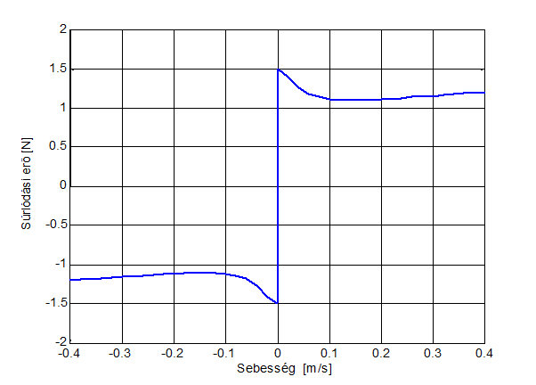
8.6.1. Stick-slip motion
A single unitary mass with friction was pulled by a spring to simulate stick-slip motion. The spring free end was moving with a constant speed. Both the speed and the stiffness of the spring was selected on such a way that stick-slip motion occurred (vspring = 0.02 m/s, kspring = 0.1 N/m). These values were the same in case of all models.
The simulation results are shown by figures from Figure 811 to Figure 815. The upper curve is the force, while the lower one is the displacement as a function of time.
Both the cases of the seven parameter, Karnopp and LuGre models we get a smooth curve. The Karnopp model does not contain time lag, thus the system responds immediately to any change. This is why the force changes over into negative value when the motion begins.
Both the modified Dahl and the M2 models show undesirable oscillations superposed on the friction force, when the mass gets stuck. However, we have to remark that the original source [33] shows a smooth curve for the M2 model. Probably that can be achieved with special parameterization.
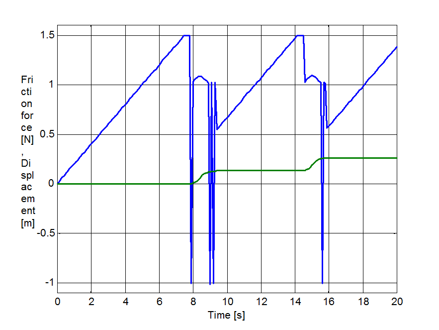
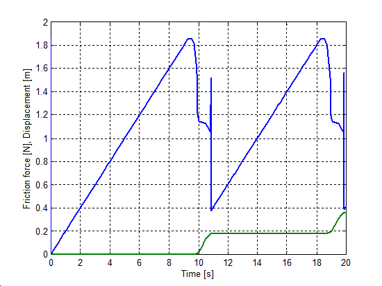
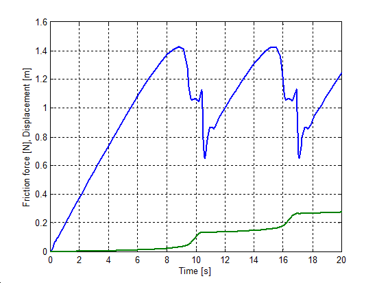
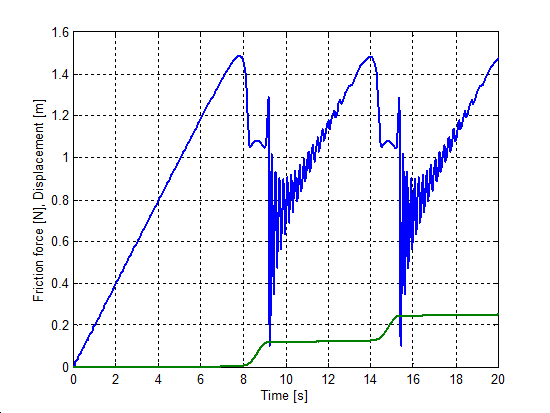
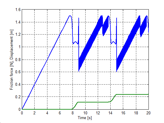
8.6.2. Zero velocity crossing
The same set up as of stick-slip was used for velocity reversals testing. The free end of the spring was pulled by a velocity changed as Asin(t), where A = 1 m/s. The simulation results plotted against time are in Figure 8-16 trough Figure 8-35 for friction force, velocity, displacement and spring force for each of the five models respectively. The thin dashed line shows the exciting velocity for all cases, except for displacement, where it is the displacement of the free spring end.
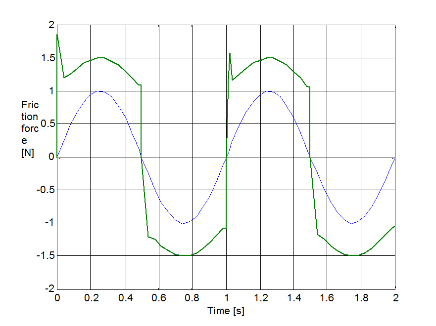
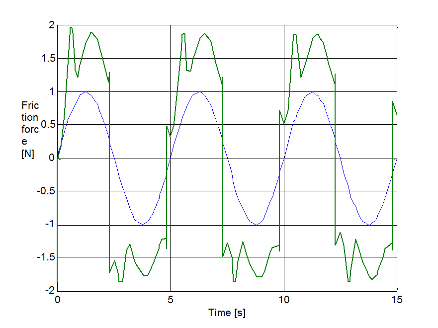
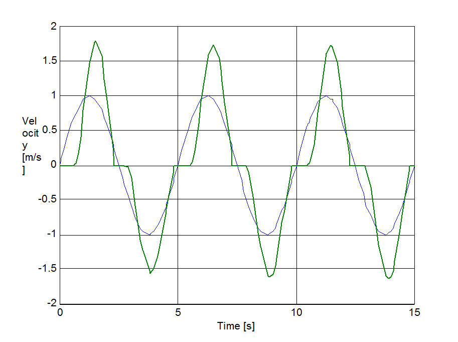
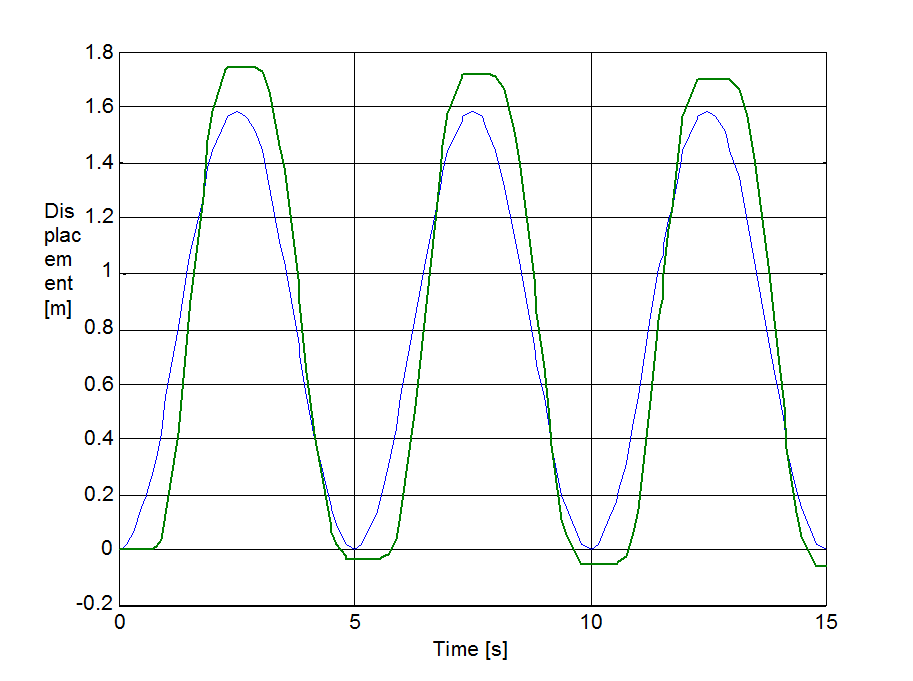
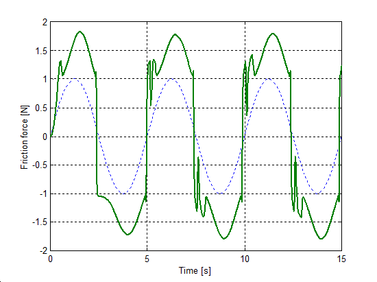
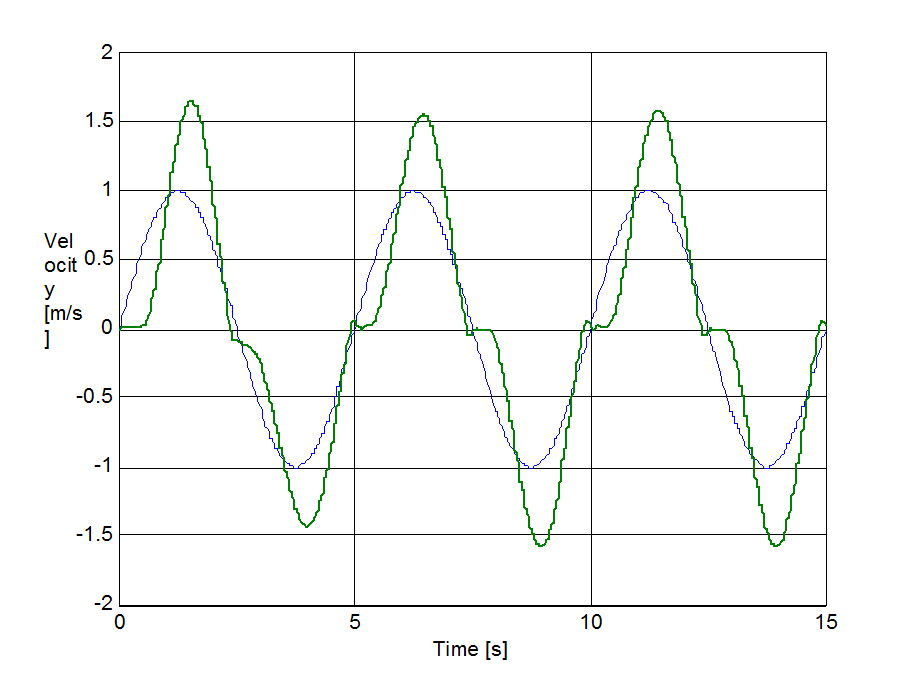
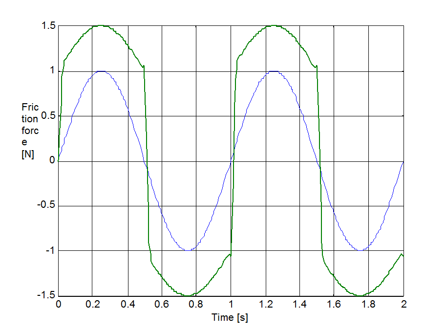
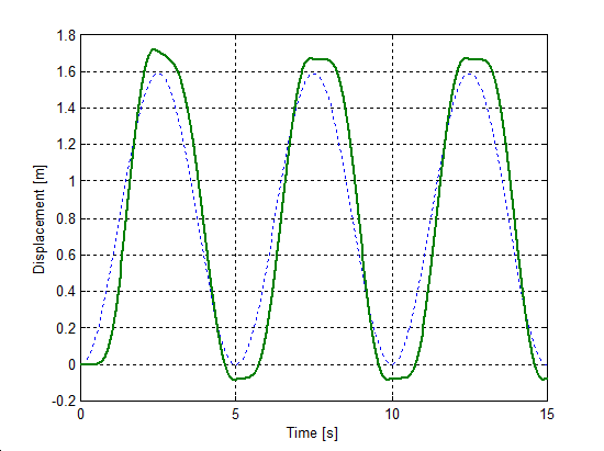
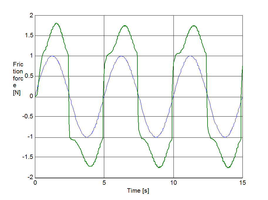
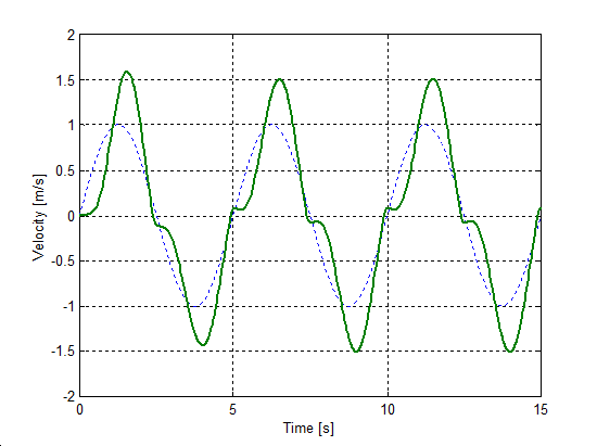
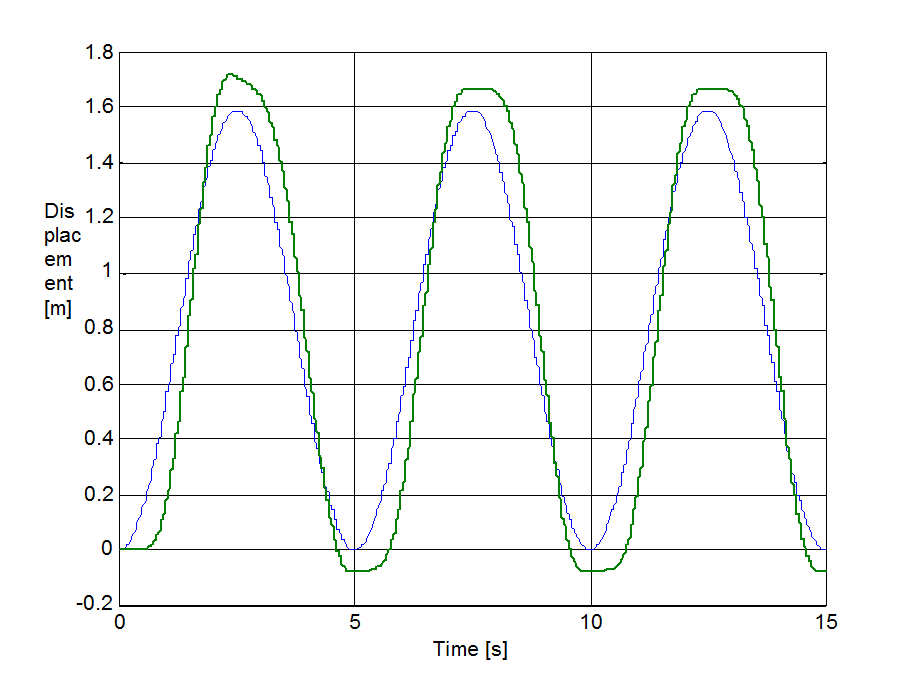
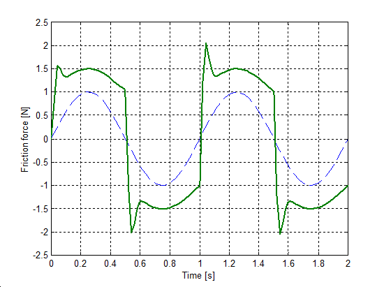
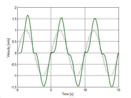

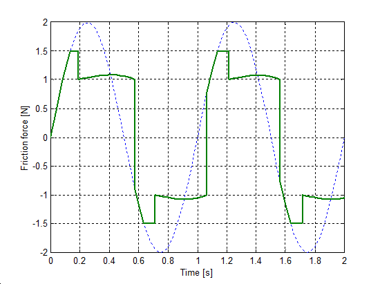
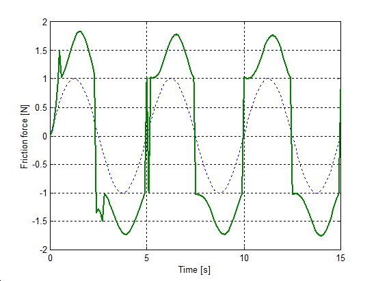
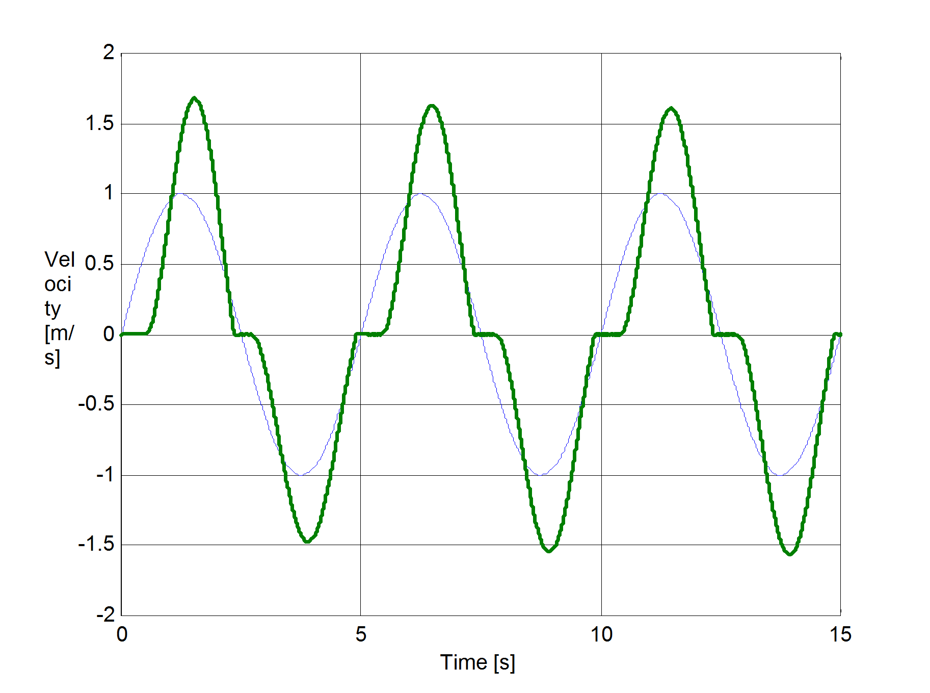

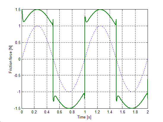
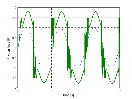
8.6.3. Spring-like stiction behavior
At zero velocities, for force excitation it is desirable that the models show the behavior of a non-linear spring. To simulate this environment a small force, less than the breakaway level was applied with the same magnitude (F = 0.5 N) in each case. The load and unload cycles were ensured by a sinus function with the given amplitude applied on the unitary mass. The resulting presliding displacement curves are in Figure 8-36–Figure 8-39. Note, that the Karnopp friction model does not contain this feature.
Unlike other models, the seven-parameters model does not show any hysteresis. The reason for that, is the seven-parameter model employs a linear spring element for modeling the Dahl effect. It is interesting to note, that the M2 model reaches its steady state only after the first cycle.
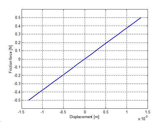
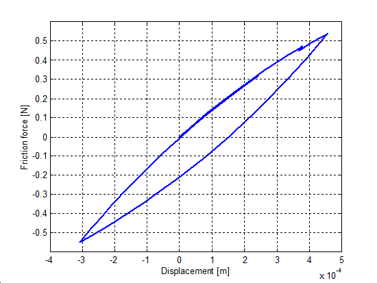
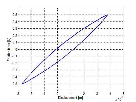
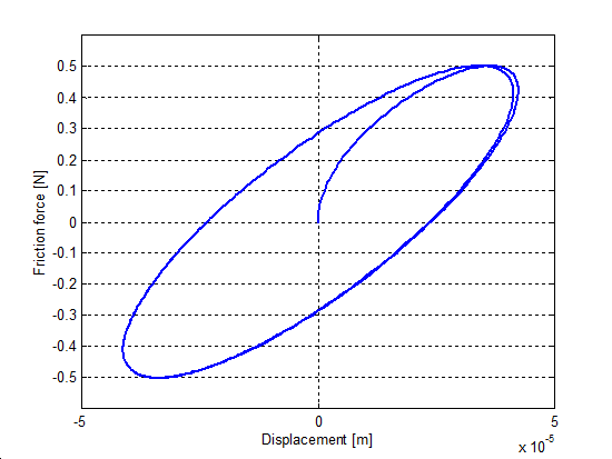
Chapter 9. PCI universal motion control system
9.1. Introduction
This manual gives instructions and technical information for system integration of the General Mechatronics PCI motion control system. The system is suitable for many servo applications like robots, CNC machines, latches, plasma cutters etc. It can be easily integrated into LinuxCNC for a complete machine control solution. (PC based motion control system. For more information, please visit the LinuxCNC official website: http://www.linuxcnc.org/)
9.2. Features and interfaces
The PCI motion control card is based on a FPGA and a PCI bridge interface ASIC. There are connectors on the whole border of the card to interface with the majority of possible system elements that can be found in an automated robotic cell.
There are six RJ50 modular axis connectors at the inner edge of the card in order to drive incremental or classic analogue servos. Four different small DIN-rail mounted axis modules are available to make possible to drive six different servo configurations in a cost effective way. The interface can be made with an exact combination of the suitable axis modules for the actual servo configuration. (See chapter 3.1.1. for the possible servo types and configurations.)
A CAN bus interface can be seen at the top edge from the right side (RJ12 modular connector): this is for modern digital servo systems which are communicating on CAN-bus.
Then in the middle, four times eight general purpose I/O pins are placed on standard flat cable headers. These bare I/O pins can be configured in LinuxCNC for any custom purpose. In most cases an optical isolation is advisable here to prevent the PCI card and the PC from disturbances and unsafe voltage transients coming from the industrial environment.
On the left side of the top edge an RS485 bus was designed to interface with compact DIN-rail mounted expander modules. An 8-channel digital input, an 8-channel relay output and an analogue I/O (4x 10 Volts output and 8x 5 Volts input) modules are available now. Maximum 16 modules can be connected to the bus altogether.
At the end, on the bottom, there is a 26 pin flat cable header with 20 optically isolated input pins. Six times three for the direct connection of two end switches and one homing sensor for each axis. Additionally, two optically isolated E-stop inputs are available.
With these functions a small automated manufacturing cell can be successfully controlled with a short time system integration procedure. The following figure demonstrates the typical connection of devices related to the control system.
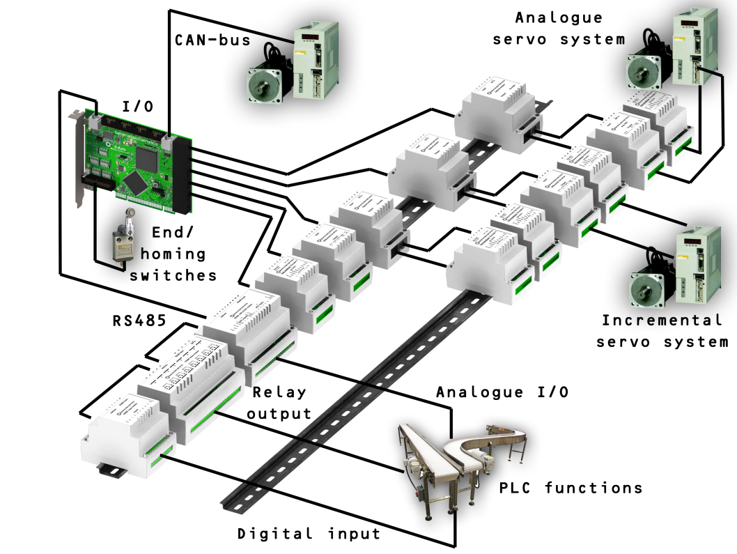
Chapter 10. PCI CARD – Specifications
- 10.1. Pin-outs and electrical characteristics
- 10.2. Mechanical dimensions
- 10.3. Connecting servo modules
- 10.4. Axis interface modules
- 10.4.1. Typical servo configurations
- 10.4.1.1. Analogue system with encoder feedback
- 10.4.1.2. Incremental digital system with encoder feedback and differential output
- 10.4.1.3. Incremental digital system with encoder feedback and TTL output
- 10.4.1.4. Incremental digital system with differential output
- 10.4.1.5. Incremental digital system with TTL output
- 10.4.1.6. Absolute digital (CAN based) system
- 10.4.1.7. Absolute digital (CAN based) system with conventional (A/B/I) encoder feedback
- 10.4.2. AXIS – Optical Isolator
- 10.4.3. AXIS – DAC (Digital-to-Analogue Converter)
- 10.4.4. AXIS – Differential breakout
- 10.4.5. AXIS – Breakout
This chapter describes all connectors, pins and the electrical characteristics of the PCI card.
10.1. Pin-outs and electrical characteristics
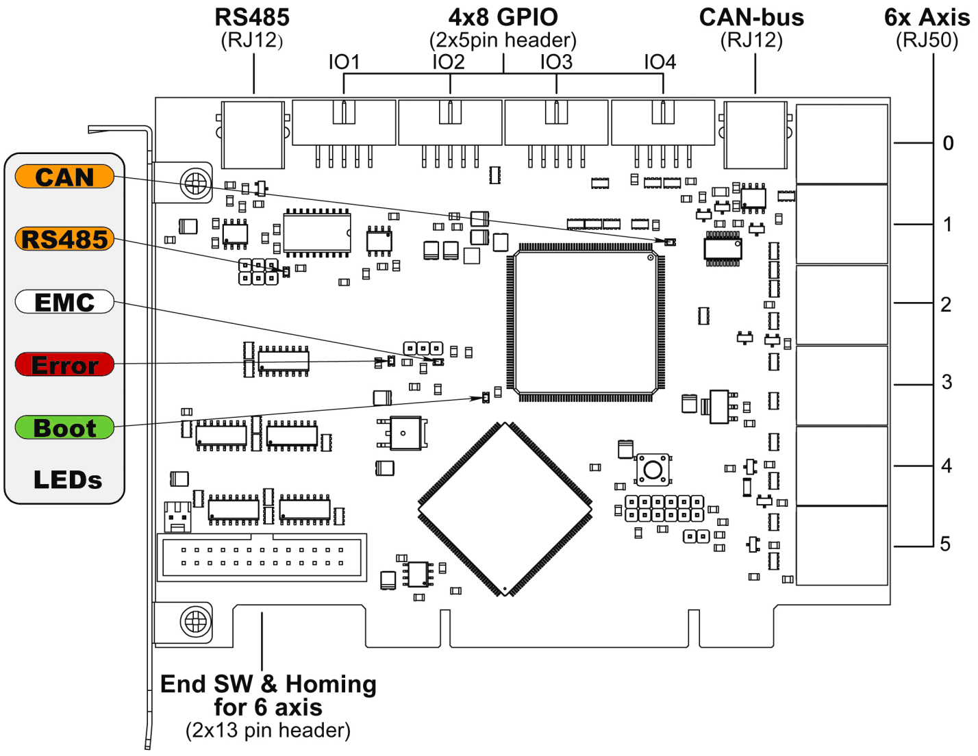
10.1.1. RS485: Extension modules
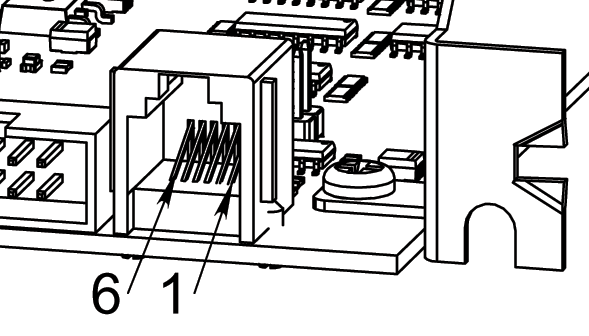
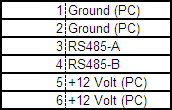
10.1.2. GPIO connectors
Each pin can be configured as digital input or output.
10.1.2.1. Pinout
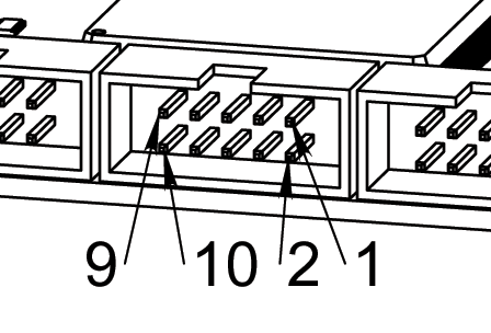
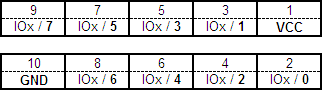
Figure 10-4. Pin numbering of GPIO connectorsFigure 10-5. Pinout of GPIO connectors
10.1.2.2. Input electrical characteristics
These are simple non-isolated I/O ports for general purpose usage. All voltage levels are referenced to the PC ground. It is not recommended to directly connect signals which can exceed the absolute maximum ratings.
Absolute maximum ratings
Maximum input voltage: 3.3Volts
Minimum input voltage: 0Volts.
Maximum current of the 4x8 output100mA
Logic levels
Minimum high-level input voltage: 2Volts
Maximum low-level input voltage:0.8Volts
10.1.2.3. Output electrical characteristics
The totem pole outputs are short circuit protected by a series resistor, see figure:

Output logic levels (unloaded)
Minimum high-level output voltage: 2.9Volts
Maximum low-level output voltage:0.4Volts
10.1.3. CAN-bus: Position reference for servo modules
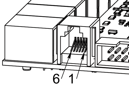
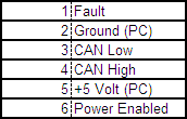
10.1.4. Axis connectors
All voltage levels on the axis connectors are referenced to the PC ground. It is recommended to use axis modules to connect the servo amplifier modules to the PCI card. See chapter 3.
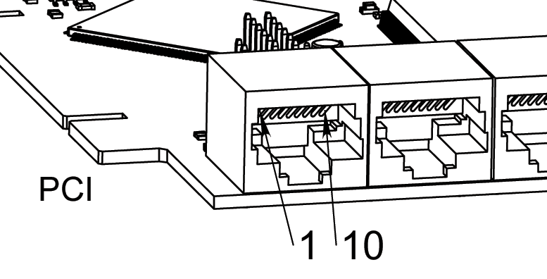
10.1.4.1. Encoder input characteristics
Absolute maximum ratings
Maximum input voltage: 3.3Volts
Minimum input voltage: 0Volts.
Logic levels
Minimum high-level input voltage: 2Volts
Maximum low-level input voltage:0.8Volts
10.1.4.2. Fault inputs
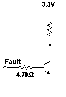
Logic levels
Minimum high-level input voltage: 1.5Volts
Maximum low-level input voltage:0.5Volts
10.1.4.3. Enabled outputs
The enable output is common for all axes.
Maximum output source current:100mA
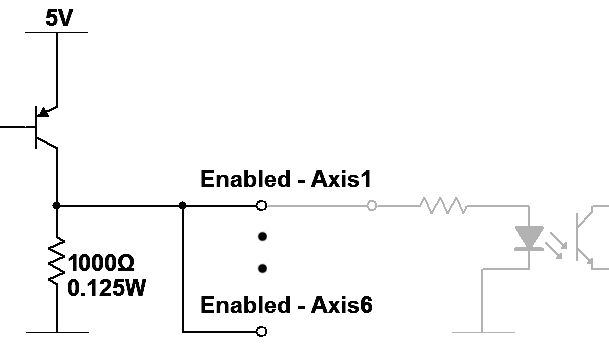
10.1.4.4. Step, Direction and DAC serial line output characteristics
The totem pole outputs are short circuit protected by a series resistor, see figure.
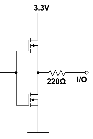
Output logic levels (unloaded)
Minimum high-level output voltage: 2.9Volts
Maximum low-level output voltage:0.4Volts
10.1.5. Homing & end switch connector
10.1.5.1. Pinout
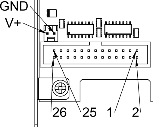
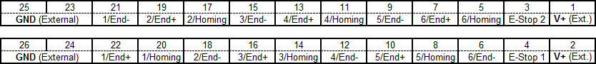
10.1.5.2. Input electrical characteristics
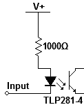
Mechanical switch or open collector output can be connected between input pins and the external ground (GND).
Logic levels referred to voltage drop between V+ , Input pins and current consumption
Minimum high-level voltage drop: 5VoltsIF3.9mA
Maximum recommended high-level voltage drop:12VoltsIF11mA
Maximum low-level voltage drop:1Volts
Absolute maximum ratings
Forward voltage drop between V+ and Input pins:30Volts
Forward current along V+ and Input pins:30mA
Reverse voltage drop between V+ and Input pins:5Volts
10.1.6. LEDs
10.1.6.1. CAN
Color: Orange
Blink, during data communication.
On, when any of the buffers are full – communication error.
Off, when there isn’t data communication.
10.1.6.2. RS485
Color: Orange
Blink, during initialization of modules on the bus
On, when the data communication is active between all initialized modules.
Off, when any of the initialized modules dropped off because of an error.
10.1.6.3. EMC
Color: White
Blink, when LinuxCNC is running.
Otherwise off.
10.1.6.4. Boot
Color: Green
On, when system booted successfully.
Otherwise off.
10.1.6.5. Error
Color: Red
Off, when there is no fault in the system.
Blink, when there is a PCI communication error.
On, when watchdog timer overflowed.
10.2. Mechanical dimensions
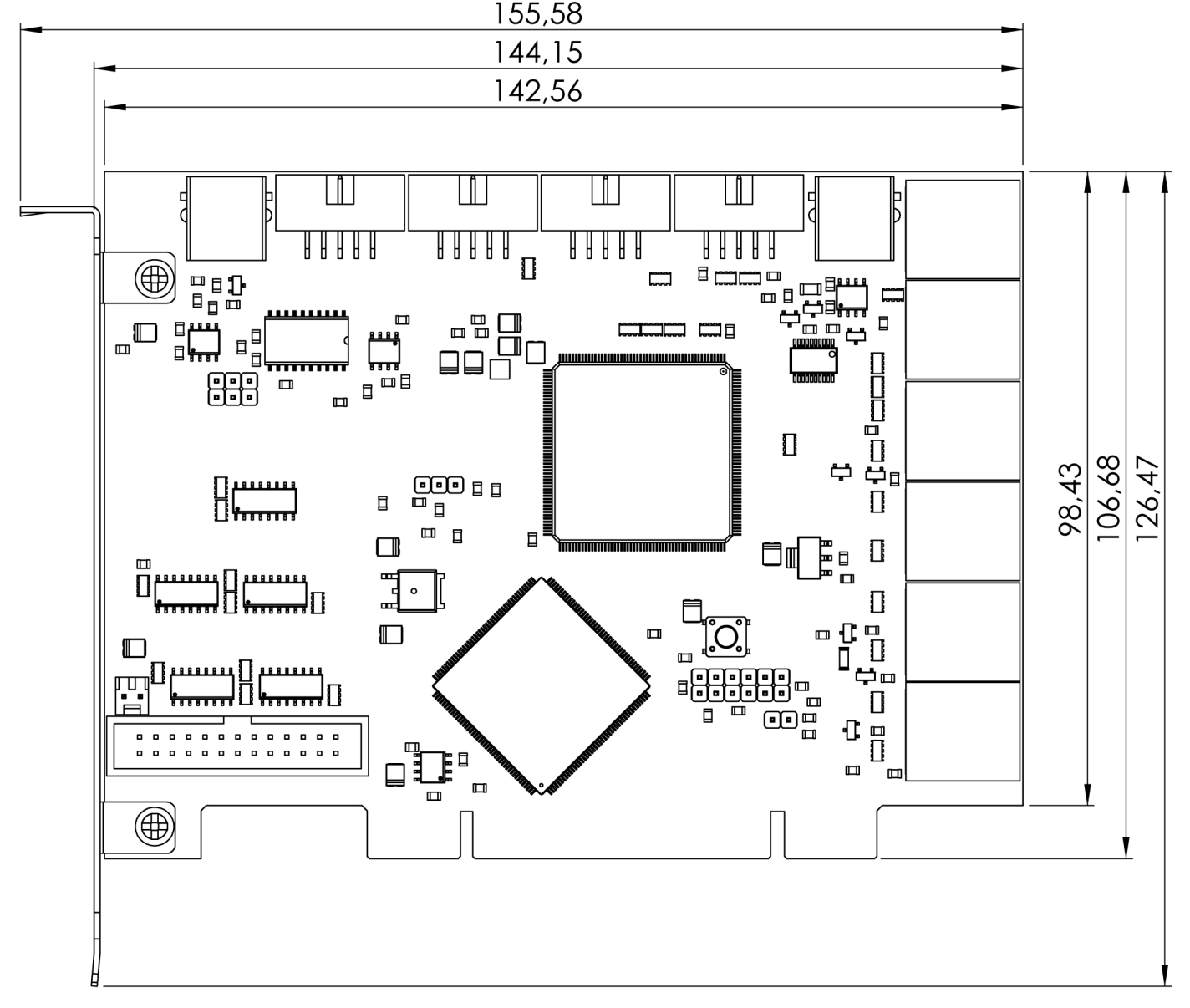
All dimensions are given in mm. Not shown dimensions are compliant with PCI specification and standard.
10.3. Connecting servo modules
This chapter is about how to connect servo modules to the PCI motion control card for driving a machine.
10.4. Axis interface modules
Small sized DIN rail mounted interface modules represent an easy way to connect different types of servo modules to the axis connectors. First in this chapter, seven different system configurations are presented that can be set up to evaluate typical applications. Then the detailed description of the four available interface modules is presented.
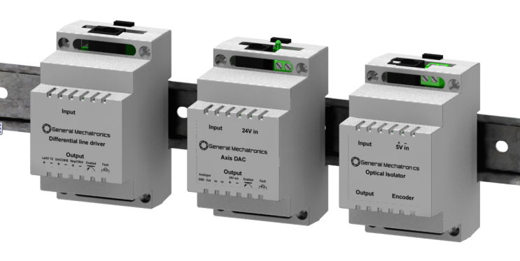
10.4.1. Typical servo configurations
In order to evaluate the appropriate servo-drive structure the modules have to be connected as it is shown in the following block diagrams. All the modular cables (RJ50 and RJ45) have to be straight wired.
10.4.1.1. Analogue system with encoder feedback
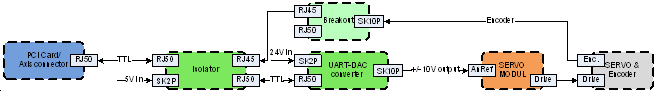
This configuration can be used to interface with the conventional analogue servo modules which have voltage level reference signal input.
10.4.1.2. Incremental digital system with encoder feedback and differential output
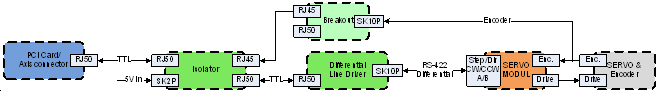
This configuration can be used to interface with three types of incremental servo modules with the following differential reference inputs: Step/Direction, Clockwise/Counter clockwise and Quadrant A/B. It is possible to read the servo position in the PC with the encoder feedback connection.
10.4.1.3. Incremental digital system with encoder feedback and TTL output
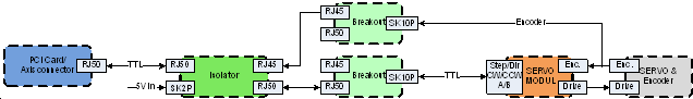
This configuration can be used to interface with three types of incremental servo modules with the following TTL level reference inputs: Step/Direction, Clockwise/Counter clockwise and Quadrant A/B. It is possible to read the servo position in the PC with the encoder feedback connection.
10.4.1.4. Incremental digital system with differential output

Same configuration as in chapter 3.1.1.2. but without isolation and encoder feedback. This configuration is recommended when the servo module has optically isolated inputs.
10.4.1.5. Incremental digital system with TTL output

Same configuration as in chapter 3.1.1.3. but without isolation and encoder feedback.
10.4.1.6. Absolute digital (CAN based) system
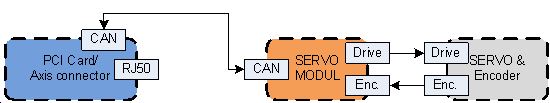
Servo modules are connected along the CAN bus interface.
10.4.1.7. Absolute digital (CAN based) system with conventional (A/B/I) encoder feedback
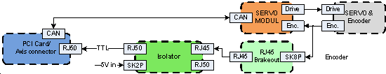
Servo modules are connected along the CAN bus interface, expanded with conventional encoder feedback along an optical isolator to the RJ50 axis connector.
10.4.2. AXIS – Optical Isolator
This module can be used to isolate all the signals referred to the PC ground, and to interface with TTL or differential output encoders. The controller side of the module can be connected to the PCI card’s Axis connector. The machine side reference output can be connected to an AXIS – Breakout module or to an AXIS – Differential breakout module, or can be hard wired directly to TTL inputs of a servo controller.
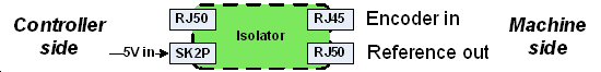
Pinout – Controller side
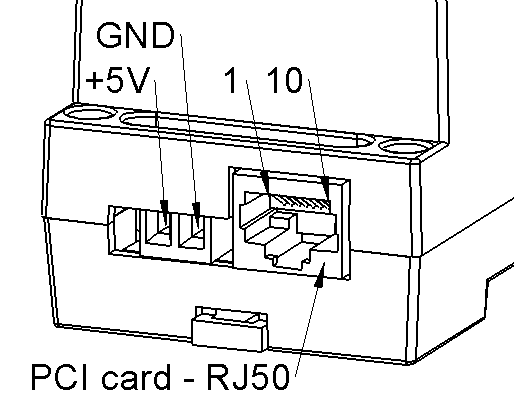
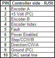
Pinout – Machine side
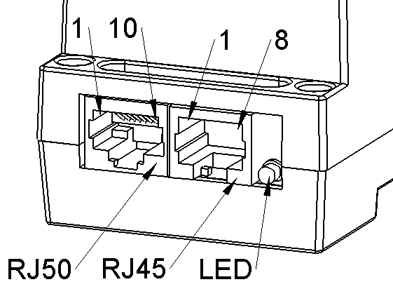
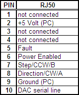
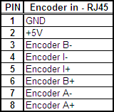
10.4.2.1.
Electrical characteristics
Output characteristics of pins on reference output (RJ50) connector:
All output pins are TTL compatible.
Maximum output high-level voltage:5Voltsno load
Minimum output high-level voltage:2VoltsIL7.5mA
Maximum output low-level voltage:0.1Volt
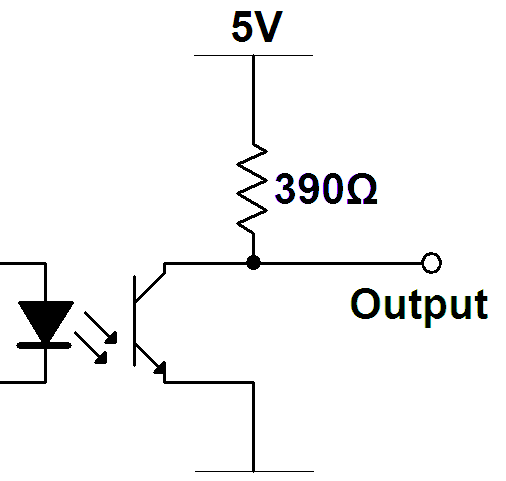
Input characteristics of fault input pin on reference output (machine side RJ50) connector:
Minimum input high-level voltage:2VoltsIF3.85mA
Maximum input low-level voltage:1Volts
Absolute maximum input voltage:7VoltsIF27mA
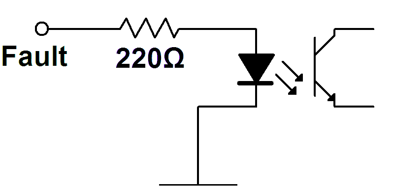
Input characteristics of pins on encoder input (RJ45) connector:
DC characteristics for differential output encoder:
Minimum high-level input voltage difference:0.2Volt
Minimum low-level input voltage difference:-0.2Volt
Maximum differential input voltage:6Volts
DC characteristics for TTL output encoder: The negative differential inputs must be left open. The outputs have to be connected to the positive inputs.
Minimum input high-level voltage:2VoltsIH110A
Maximum input low-level voltage:1.2Volts IL-110A
Maximum frequency at symmetrical square signal:500kHz
Maximum load current of encoder power:500mA
Input DC characteristics of pins on PCI card – RJ50 (controller side) connector:
Minimum input high-level voltage:2VoltsIF3.85mA
Maximum input low-level voltage:1Volts
Absolute maximum input voltage:7VoltsIF27mA
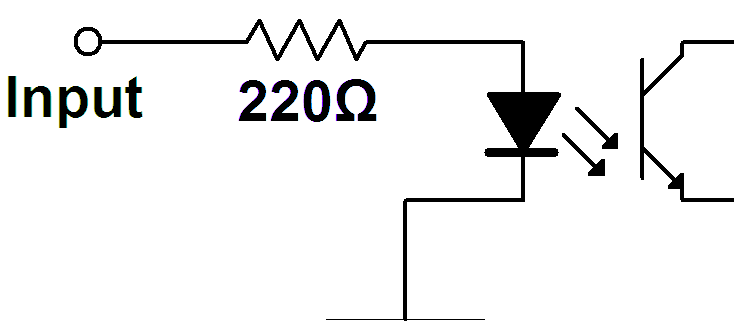
Output DC characteristics of Fault output pin on PCI card – RJ50 (controller side) connector:
Maximum output high-level voltage:5Voltsno load
Minimum output high-level voltage:2VoltsIL7.5mA
Maximum output low-level voltage:0.8VoltIL-360A
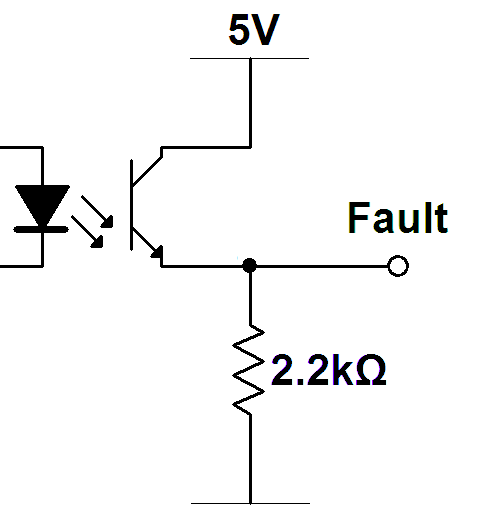
Supply voltage:
Recommended supply voltage:5Volts
Absolute maximum supply voltage:5.5Volts
Absolute minimum supply voltage:4.5Volts
Maximum current consumption without encoder:200mA
Maximum current consumption with encoder:750mA
10.4.3. AXIS – DAC (Digital-to-Analogue Converter)
This module converts the digital signal of the PCI card to analogue output to drive a speed or current mode servo amplifier. The isolator module is recommended in most cases to be used with this module, see chapter 3.1.1.1. “Analogue system with encoder feedback”.
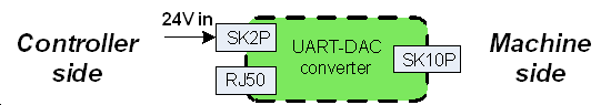
The controller side RJ50 connector of this module has to be connected to the machine side of an AXIS – Optical Isolator module or directly to the PCI card (when the servo amplifier is isolated). The machine side terminal output can be connected to an analogue type servo amplifier.
Controller side pinout
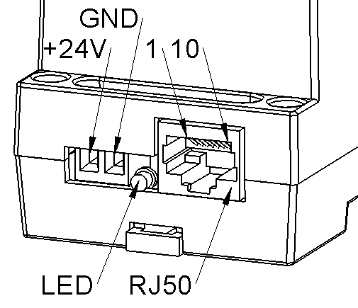
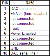
Machine side pinout

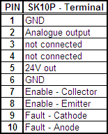
Electrical characteristics
Controller side RJ50 connector:
Serial line in single line connection – only serial line+ is connected (most cases):
Serial line+ minimum high level input voltage:3Volts
Serial line+ maximum low level input voltage:2Volts
Serial line in differential connection:
Minimum high level input voltage difference:0.4Volts
Maximum low level input voltage difference:0.4Volts
Fault signal – open emitter output signal:
Maximum high level output voltage:5Volts
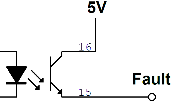
Enabled input signal
Minimum high level input voltage:2Volts
Maximum low level input voltage:0.8Volts
Machine side terminal connector:
DAC output:
Maximum output voltage:10Volts
Minimum output voltage:-10Volts
Output voltage level accuracy:1%
24V output:
Maximum output load current:200mA
Enabled output signal:
Collector-emitter breakdown voltage:80VoltsIC0.5mA
Emitter-collector breakdown voltage:7VoltsIE0.1mA
Maximum collector dark current:0.1AVCE48Volts
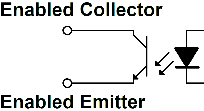
For more information please refer to Toshiba TLP281 optocoupler’s datasheet.
Fault input signal - LED:
LED forward voltage:1.15VoltsIF10mA
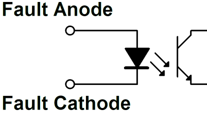
For more information please refer to Toshiba TLP281 optocoupler’s datasheet.
Operating conditions
The following conditions have to be fulfilled to have the analogue voltage level and enabled signal at the output in order to drive the analogue servo module:
External 24 Volt DC supply is connected and the digital part is supplied with 5 Volts from the isolator or from the PCI card.
No watchdog error
No DAC voltage level fault
The valid digital reference signal comes on UART from the PC
No servo fault - The fault signal from the servo module is LOW
Drive enabled - Enabled signal from the PC is HIGH
Fault conditions
The following flowchart describes the fault handling of the axis DAC module:

Watchdog reset occurred:
- LED blinks continuously
- The fault signal from the servo module is overdriven to HIGH
- The Enabled signal to the servo module is overdriven to LOW
- The analogue output is equal to 0 Volt.
- Reversed when enable signal from PC is turned off and then turned on again, or power reset occurred.
DAC output voltage level is not equal to the specified voltage (DAC error):
- LED blinks once every second
- The fault signal from the servo module is overdriven to HIGH
- The Enabled signal to the servo module is overdriven to LOW
- The analogue output is equal to 0 Volt.
- Reversed on power reset. If the error still remains, replace the DAC module.
No digital input or the UART frame is broken:
- LED blinks twice every second
- The fault signal from the servo module is overdriven to HIGH
- The Enabled signal to the servo module is overdriven to LOW
- The analogue output is equal to 0 Volt.
- Reversed when digital input signal on UART line becomes valid again.
Fault signal from servo module is HIGH:
- LED blinks tree times every second
- The analogue output is equal to 0 Volt.
- Reversed when fault signal becomes LOW again.
Enabled signal from PC is LOW:
- LED is off.
- The analogue output is equal to 0 Volt.
- Reversed when enabled signal becomes HIGH again.
10.4.4. AXIS – Differential breakout
This module can be used to interface with servo modules which have differential reference input.
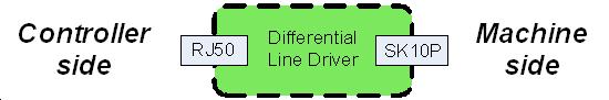
The controller side can be connected directly to the PCI card’s axis connector if there is no need for optical isolation or encoder feedback to the controller. In any other cases the controller side should be connected to the machine side RJ50 connector of an AXIS – Optical Isolator module.
Controller side pinout
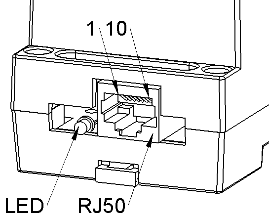
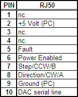
Machine side pinout

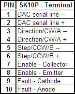
Electrical characteristics
Controller side RJ50 connector:
TTL inputs (pins: 6, 7, 8, 10):
Minimum high level input voltage:2Volts
Maximum low level input voltage:0.8Volts
For more information please refer to AM26LS31 differential line driver’s datasheet.
Machine side terminal connector:
Differential outputs:
Maximum low level output current:20mA
Maximum high level output current:-20mA
For more information please refer to AM26LS31 differential line driver’s datasheet.
Enabled output signal:
Collector-emitter breakdown voltage:80VoltsIC0.5mA
Emitter-collector breakdown voltage:7VoltsIE0.1mA
Maximum collector dark current:0.1AVCE48Volts

For more information please refer to Toshiba TLP281 optocoupler’s datasheet.
Fault input signal - LED:
LED forward voltage:1.15VoltsIF10mA
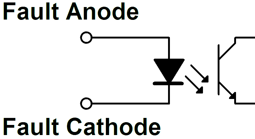
For more information please refer to Toshiba TLP281 optocoupler’s datasheet.
10.4.5. AXIS – Breakout
This module can be used for wiring out the reference outputs or the encoder inputs modular contacts to a simple terminal connector. In case of the encoder it can be useful to split the signals between the servo module and the encoder feedback to the PC.
Connectors
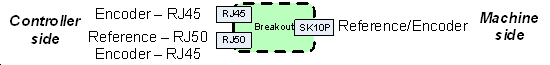
Controller side RJ50 & RJ45 modular connectors
The 10-pin RJ50 connector can also host 8-pin RJ45 plug. In case of splitting the encoder signals, two RJ45 encoder cables can be used.
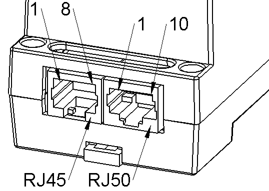
Controller side RJ50 – Reference or Encoder pinout:
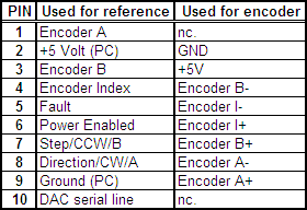
Controller side RJ45 – Encoder pinout:
The power supply of the encoder is not connected on the secondary (RJ45) connector to ensure that the encoder sensor gets the supply voltage from one source only.
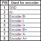
Machine side SK10P - Terminal connector pinout:
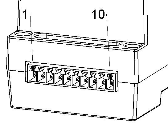
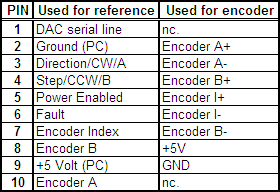
Chapter 12. HAL settings
In this chapter, all the relevant system relevant hall settings can be found, except for the modules on the RS485 bus. Those can be found in the next chapter for each module.
All the pins and parameters of this chapter are updated by the following two functions:
gm.<nr. of card>.read
gm.<nr. of card>.write
Both should be added to the servo thread in this given order (first read then write) for most applications.
12.1. Encoder
The motion control card has six encoder modules. Each encoder module has three channels:
Channel-A
Channel-B
Channel-I (index).
The encoder is able to count quadrature encoder signals or step/dir signals. Each encoder module is connected to the inputs of the corresponding RJ50 axis connector.
Every encoder pin and parameter name begins as follows:
gm.<nr. of card>.encoder.<nr of axis>,where <nr of axis> is form 0 to 5.
For example: gm.0.encoder.0.position►refers to the position of the encoder module of axis 0.
The PCI card counts the encoder signal independently from LinuxCNC.
HAL pins are updated by the gm.<nr of card>.read function.
12.1.1. Pins:
.reset(bit, In)► When True, resets counts and position to zero.
.rawcounts(s32, Out)► The raw count is similar to the counts, but unaffected by reset or the index pulse.
.counts(s32, Out)► Position in encoder counts.
.position(float, Out)► Position in scaled units (=.counts/.position-scale).
.index-enabled(bit, IO) ►When True, counts and position are rounded or reset (depends on index-mode) on next rising edge of channel-I. Every time position is reset because of Index, the index-enabled pin is set to 0 and remain 0 until the connected HAL pin does not set it.
.velocity (float, Out) ► Velocity in scaled units per second. GM encoder uses high frequency hardware timer to measure the time between encoder pulses in order to compute velocity. It greatly reduces quantization noise as compared to simply differentiating the position output. When the measured velocity is below min-velocity-estimate, the velocity output is 0.
12.1.2. Parameters:
.counter-mode(bit, R/W)► When True, the counter counts each rising edge of the channel-A input to the direction determined by channel-B. This is useful for counting the output of a single channel (non-quadrature) or step/dir signal sensor. When false, it counts in quadrature mode.
.index-mode(bit, R/W)► When True and .index-enabled is also true, .counts and .position are rounded (based on .counts-per-rev) at rising edge of channel-I. This is useful to correct few pulses error caused by noise. In round mode, it is essential to set .counts-per-rev parameter correctly. When .index-mode is False and .index-enabled is true, .counts and .position are reset at channel-I pulse.
.counts-per-rev(u32, R/W)► Determine how many counts are between two index pulses. It is used only in round mode, when both .index-enabledand.index-mode parameters are True. GM encoder process encoder signal in 4x mode, so for example in case of a 500 CPR encoder it should be set to 2000. This parameter can be easily measured by setting .index-enabledtoTrue and .index-mode to False (so that .counts resets at channel-I pulse), than move the axis by hand and see the maximum magnitude of .counts pin in halmeter.
.index-invert(bit, R/W)► When True, channel-I event (reset or round) occur on the falling edge of channel-I signal, otherwise on the rising edge.
.min-speed-estimate(float, R/W)► Determine the minimum measured velocity magnitude at which .velocity will be set as nonzero. Setting this parameter too low will cause it to take a long time for velocity to go to zero after encoder pulses have stopped arriving.
.position-scale(float, R/W)►Scale in counts per length unit. .position=.counts/.position-scale. For example, if position-scale is 2000, then 1000 counts of the encoder will produce a position of 0.5 units.
12.1.3. HAL example
Setting encoder module of axis 0 to receive 500 CPR quadrature encoder signal and use reset to round position:
setp gm.0.encoder.0.counter-mode 0# 0: quad, 1: stepDir
setp gm.0.encoder.0.index-mode 1# 0: reset pos at index, 1:round pos at index
setp gm.0.encoder.0.counts-per-rev 2000# GM process encoder in 4x mode, 4x500=2000
setp gm.0.encoder.0.index-invert 0
setp gm.0.encoder.0.min-speed-estimate 0.1#in position unit/s
setp gm.0.encoder.0.position-scale 20000#in case of 10 encoder revolutions cause the machine to move one position unit (10x2000)
Connect encoder position to LinuxCNC position feedback:
net Xpos-fb gm.0.encoder.0.position => axis.0.motor-pos-fb
12.2. Stepgen module
The motion control card has six stepgen modules, one for each axis. Each module has two output signals. It can produce Step/Direction, Up/Down or Quadrature (A/B) pulses. Each stepgen module is connected to the pins of the corresponding RJ50 axis connector.
Every stepgen pin and parameter name begins as follows:
gm.<nr. of card>.stepgen.<nr of axis>, where nr of axis is from 0 to 5.
For example: gm.0.stepgen.0.position-cmd►refers to the position command of stepgen module of axis 0 on card 0.
The PCI card generates step pulses independently from LinuxCNC. HAL pins are updated by gm.<nr of card>.write function.
12.2.1. Pins:
.enable(bit, In)► Stepgen produces pulses only when this pin is true.
.count-fb(s32, Out)► Position feedback in count units.
.position-fb(float, Out)► Position feedback in position units.
.position-cmd(float, In)► Commanded position in position units.
Used in position mode only.
.velocity-cmd(float, In)► Commanded velocity in position units per second.
Used in velocity mode only.
12.2.2. Parameters:
.step-type(u32, R/W)►When 0, the module produces Step/Dir signal.
When 1, it produces Up/Down step signals. And when it is 2, it produces quadrature output signals.
.control-type(bit, R/W)►When True, .velocity-cmd is used as reference and the velocity control computes pulse rate output. When False, .position-cmd is used as reference and position control calculate pulse rate output.
.invert-step1(bit, R/W)►Invert the output of channel 1.
(Step signal in StepDir mode)
.invert-step2(bit, R/W)►Invert the output of channel 2.
(Dir signal in StepDir mode)
.maxvel(float, R/W)► Maximum velocity in position units per second.
If it is set to 0.0, .maxvel parameter is ignored.
.maxaccel(float, R/W)►Maximum acceleration in position units per second squared. If it is set to 0.0, .maxaccel parameter is ignored.
.position-scale(float, R/W)►Scale in steps per length units.
.position-fb=.count-fb/.position-scale. For example, if position-scale is 1000, then 1 position unit command produces 1000 step pulses.
.steplen(u32, R/W)►Length of step pulse in nano-seconds.
.stepspace(u32, R/W)►Minimum time between two step pulses in nano-seconds.
.dirdelay(u32, R/W)►Minimum time between step pulse and direction change in nano-seconds.
In order to evaluate the appropriate values see the timing diagrams below:
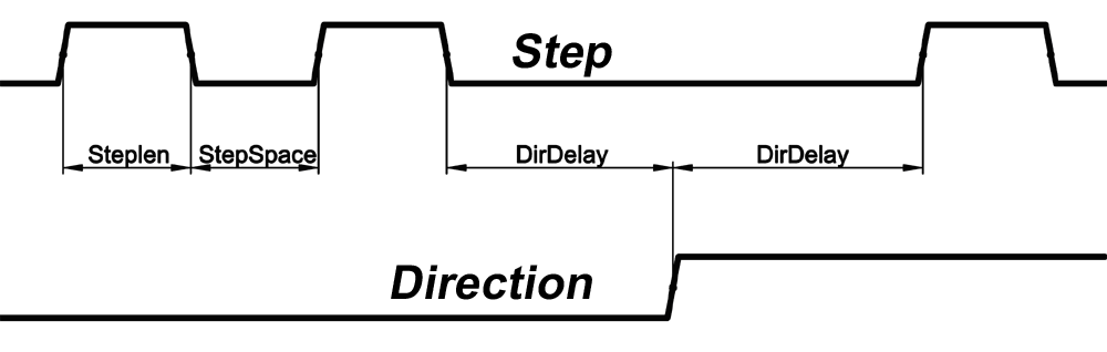
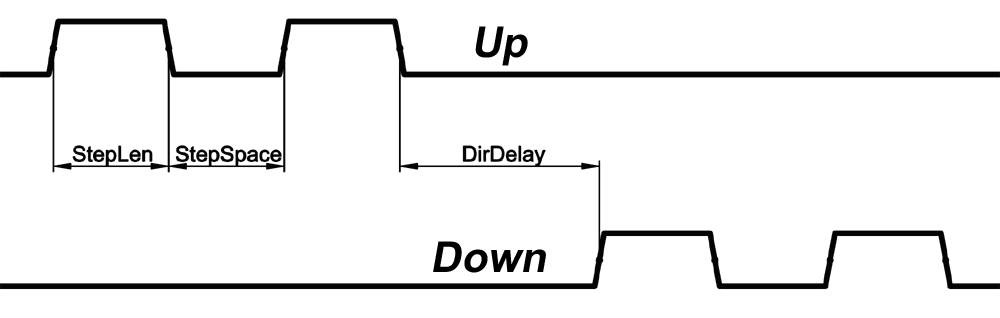
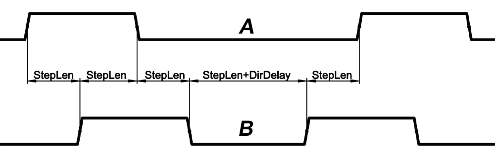
12.2.3. HAL example:
Setting stepgen module of axis 0 to generate 1000 step pulse per position unit:
setp gm.0.stepgen.0.step-type 0# 0:stepDir,1:UpDown,2:Quad
setp gm.0.stepgen.0.control-type 0# 0:Pos. control, 1:Vel. control
setp gm.0.stepgen.0.invert-step1 0
setp gm.0.stepgen.0.invert-step2 0
setp gm.0.stepgen.0.maxvel 0# do not set maxvel for the step generator, let the interpolator control it.
setp gm.0.stepgen.0.maxaccel 0# do not set max acceleration for the step generator, let the interpolator control it.
setp gm.0.stepgen.0.position-scale 1000# 1000 step/position units
setp gm.0.stepgen.0.steplen 1000 # 1000 ns = 1 us
setp gm.0.stepgen.0.stepspace1000# 1000 ns = 1 us
setp gm.0.stepgen.0.dirdelay 2000# 2000 ns = 2 us
Connect stepgen to axis 0 position reference and enable pins:
net Xpos-cmd axis.0.motor-pos-cmd => gm.0.stepgen.0.position-cmd
net Xen axis.0.amp-enable-out => gm.0.stepgen.0.enable
12.3. Axis DAC (digital-to-analogue converter)
The motion control card has six serial axis DAC driver modules, one for each axis. Each module is connected to the pin of the corresponding RJ50 axis connector.
Every axis DAC pin and parameter name begins as follows:
gm.<nr. of card>.dac.<nr of axis>,where nr of axis is from 0 to 5.
For example:gm.0.dac.0.value►refers to the output voltage of DAC module of axis 0.
HAL pins are updated by gm.<nr of card>.write function.
12.3.1. Pins:
.enable(bit, In)►Enable DAC output. When enable is false, DAC output is 0.0 V.
.value(float, In)► Value of DAC output in Volts.
12.3.2. Parameters:
.offset(float, R/W)►Offset is added to the value before the hardware is updated
.high-limit(float, R/W)►Maximum output voltage of the hardware in volts.
.low-limit(float, R/W)►Minimum output voltage of the hardware in volts.
.invert-serial(float, R/W)►PCI card is communicating with DAC hardware via fast serial communication to highly reduce time delay compared to PWM. DAC module is recommended to be isolated which is negating serial communication line. In case of isolation, leave this parameter to default (0), while in case of none-isolation, set this parameter to 1.
12.4. Enable and Fault signals
The PCI motion control card has one enable output and one fault input HAL pins, both are connected to each RJ50 axis connector and to the CAN connector.
HAL pins are updated by gm.<nr of card>.read function.
12.4.1. Pins:
gm.<nr of card>.power-enable(bit, In)►If this pin is True,
and Watch Dog Timer is not expired
and there is no power fault
Then power enable pins of axis- and CAN connectors are set to high, otherwise set to low.
gm.<nr of card>.power-fault(bit, Out)►Power fault input
12.5. Watchdog timer
Watchdog timer resets at gm.<nr of card>.read function.
12.5.1. Pins:
gm.<nr of card>.watchdog-expired(bit, Out)►Indicates that watchdog timer is expired.
Watchdog timer overrun causes the set of power-enable to low in hardware.
12.5.2. Parameters:
gm.<nr of card>.watchdog-enable(bit, R/W)►Enable watchdog timer.
It is strongly recommended to enable watchdog timer, because it can disable all the servo amplifiers by pulling down all enable signal in case of PC error.
gm.<nr of card>.watchdog-timeout-ns(u32, R/W)►Time interval in which the gm.<nr of card>.readfunction must be executed. The gm.<nr of card>.read is typically added to servo-thread, so watch timeout is typically set to 3 times the servo period.
12.6. GM-CAN
The motion control card has a CAN module to drive CAN servo amplifiers. Implementation of higher level protocols like CAN open is further development. Currently GM produced power amplifiers have upper level drivers which export pins and parameters to HAL. They receive position reference and provide encoder feedback via CAN bus.
Every CAN pin and parameter name begins as follows:
gm.<nr. of card>.can-gm.<nr of axis>,where <nr of axis> is from 0 to 5.
For example:gm.0.can-gm.0.position►refers to the output position of axis 0 in position units.
HAL pins are updated by gm.<nr of card>.write function.
12.6.1. Pins:
.enable(bit, In)►Enable sending position references
.position-cmd(float, In)►Commanded position in position units.
.position-fb(float, Out)►Feed back position in position units.
12.6.2. Parameters:
.position-scale(float, R/W)►Scale in per length units.
.position-fb=.encoder-counts/.position-scale. For example, if position-scale is 1000, then 2000 encoder pulses on GM power amplifier produces 2 on position-fb pin.
12.7. Home and Limit switches
The PCI motion control card has two limit- and one homing switch input for each axis. All the names of these pins begin as follows:
gm.<nr. of card>.axis.<nr of axis>,where nr of axis is from 0 to 5.
For example:gm.0.axis.0.home-sw-inindicates the state of the axis 0 home switch.
HAL pins are updated by gm.<nr of card>.read function.
12.7.1. Pins:
.home-sw-in(bit, Out)► Home switch input
.home-sw-in-not(bit, Out)► Negated home switch input
.neg-lim-sw-in(bit, Out)► Negative limit switch input
.neg-lim-sw-in-not(bit, Out)► Negated negative limit switch input
.pos-lim-sw-in(bit, Out)► Positive limit switch input
.pos-lim-sw-in-not(bit, Out)► Negated positive limit switch input
12.8. Emergency stop input signals
In addition to home and limit switches, there are two emergency stop (E-Stop) inputs to detect if the E-Stop button is pressed.
12.8.1. Pins:
gm.0.estop.0.in-0(bit, Out)► Estop 0 input
gm.0.estop.0.in-not-0(bit, Out)► Negated Estop 0 input
gm.0.estop.0.in-1(bit, Out)► Estop 1 input
gm.0.estop.0.in-not-1(bit, Out)► Negated Estop 1 input
12.9. General purpose I/O
The GM 6 axis motion control card has 4 general purpose I/O (GPIO) connectors, with eight configurable I/O c onnectors on each.
Every GPIO pin and parameter name begins as follows:
gm.<nr. of card>.gpio.<nr of gpio con>,where <nr of gpio con> is from 0 to 3.
For example:gm.0.gpio.0.in-0 indicates the state of the first pin of the first GPIO connector on the PCI card.
HAL pins are updated by gm.<nr of card>.read function.
12.9.1. Pins:
.in-<0-7>(bit, Out)►Input pin
.in-not-<0-7>(bit, Out)►Negated input pin
.out-<0-7>(bit, In)►Output pin. Used only when GPIO is set to output.
12.9.2. Parameters:
.is-out-<0-7>(bit, R/W)►When True, the corresponding GPIO is set to the totem-pole output, other wise is set to high impedance input.
.invert-out-<0-7>(bit, R/W)►When True, the pin value will be inverted. Is used when the pin is configured as output.
Chapter 13. RS485 modules
These modules were developed to expand the I/O and function capabilities along an RS485 line of the PCI motion control card.
13.1. Available module types
8-channel relay output module
The relay output module provides eight NO-NC relay output on a three pole terminal connector for each channel.
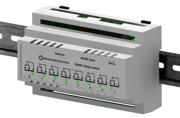
8-channel digital input module
The digital input module provides eight optical isolated digital input pins.
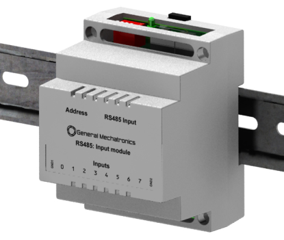
8 channel ADC and 4-channel DAC module
The ADC and DAC module provides four digital-to-analogue converter outputs and eight analogue-to-digital inputs. This module is also optically isolated from the PCI card.
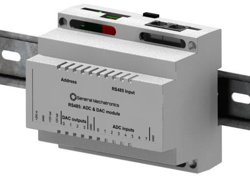
Teach Pendant module
The teach pendant module provides 8 digital input channels for pushbuttons, 6 ADC input channels for joystick or potentiometers and 1 encoder input for a handwheel.
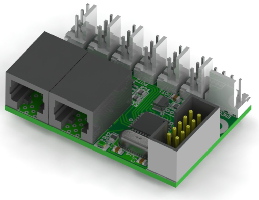
13.2. Automatic node recognizing
Each node connected to the bus is recognized by the PCI card automatically. During starting LinuxCNC, the driver exports pins and parameters of all available modules automatically.
13.3. Fault handling
If a module does not answer regularly the PCI card drops down the module.
If a module with output don’t get data with correct CRC regularly, the module switch to error state (green LED blinking), and turns all outputs to error sate.
13.4. System description
13.4.1. Powering of the nodes
Each module is electronically isolated from the bus, hence they have a bus powered side, and a field powered side.
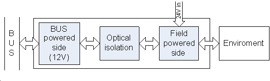
General bus settings

13.4.2. Connecting of the nodes
The modules on the bus have to be connected in serial topology, with termination resistors on the end. The start of the topology is the PCI card, and the end is the last module.
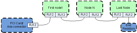
13.4.3. Addressing
Each node on the bus has a 4 bit unique address that can be set with the red DIP switch.
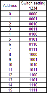
13.4.4. Status LED
The green LED indicates the status of the module:
Blink, when the module is only powered, but not yet identified, or when the module is dropped down.
Off, during identification (computer is on, but LinuxCNC not started)
On, when it communicates continuously.
13.5. Modules
13.5.1. Relay output module
Block diagram
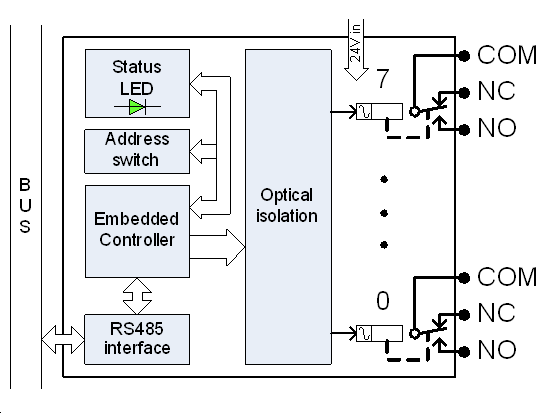
Electrical characteristics
Power:
Bus voltage:12V
Maximum bus power consumption:150mA
Field power voltage:24V
Maximum field power consumption (all relays on):270mA
Insulation:
Optical isolation voltage:2500VRMS
Relay characteristics:
Maximum switching current:10A
Maximum switching AC voltage:250V
Maximum switching DC voltage:30V
Dielectric strength:5000V
Connection
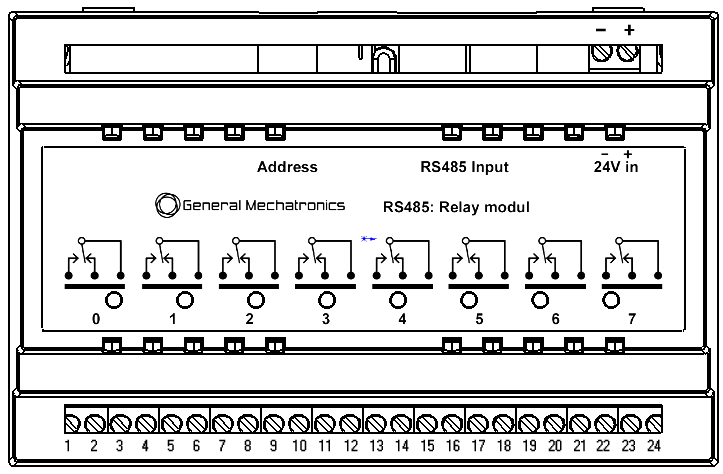
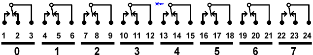
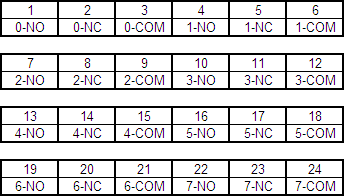
Error state
If a bus error occurs, the module will switch to error state (green LED blinking). And turn off all output relays.
HAL configuration
All the pins and parameters are updated by the following function:
gm.<nr. of card>.rs485
It should be added to servo thread or other thread with larger period to avoid CPU overload.
Every RS485 module pin and parameter name begins as follows:
gm.<nr. of card>.rs485.<modul ID>, where <modul ID> is from 00 to 15.
Pins:
.relay-<0-7>(bit, Out)--Output pin for relay
Parameters:
.invert-relay-<0-7>(bit, R/W)--Negate relay output pin
For example:
gm.0.rs485.0.relay-0– First relay of the node.
gm.0 – Means the first PCI motion control card (PCI card address = 0)
.rs485.0 – Select node with address 0 on the RS485 bus
.relay-0 – Select the first relay
13.5.2. Digital input module
Block diagram
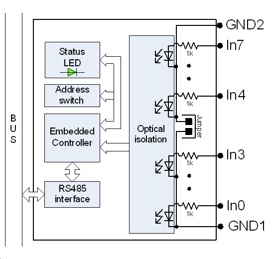
Electrical characteristics
Power:
Bus voltage:12V
Bus power consumption:100mA
Insulation:
Optical isolation voltage:2500VRMS
Input characteristics:
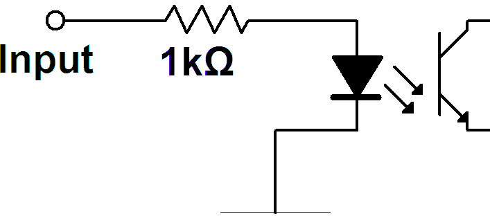
Absolute maximum ratings
Maximum input voltage: 30Volts
Minimum input voltage: -4Volts.
Maximum input current30mA
Logic levels
Minimum high-level input voltage: 5Volts
Maximum low-level input voltage:0.6Volts
For more information please refer to Toshiba TLP281 optocoupler’s datasheet.
Connection
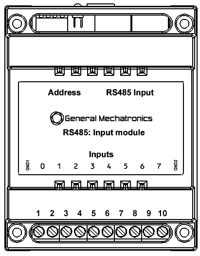

LinuxCNC HAL configuration
All the pins and parameters are updated by the following function:
gm.<nr. of card>.rs485
It should be added to the servo thread or other thread with larger period to avoid CPU overload.
Every RS485 module pin and parameter name begins as follows:
gm.<nr. of card>.rs485.<modul ID>, where <modul ID> is from 00 to 15.
Pins:
.in-<0-7>(bit, Out)--Input
.in-not-<0-7>(bit, Out)--Negated input
For example:
gm.0.rs485.0.in-0– First input of the node.
gm.0 – Means the first PCI motion control card (PCI card address = 0)
.rs485.0 – Select node with address 0 on the RS485 bus
.in-0 – Select the first digital input module
13.5.3. ADC & DAC module
Block diagram
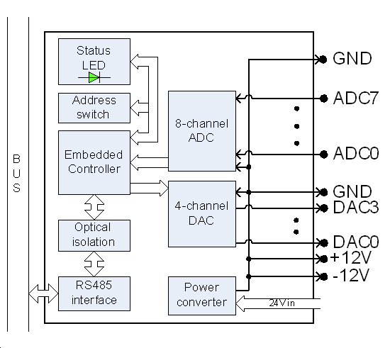
Electrical characteristics
Power:
Bus voltage:12V
Bus power consumption:100mA
Field power voltage:24V
Maximum field power consumption:500mA
Insulation:
Optical isolation voltage:2500VRMS
AD converter:
Input voltage range:5V
Input resistance:820k
Input capacitance:2nF
DA converter:
Output voltage range:10V
Maximum output current:20mA
Connection
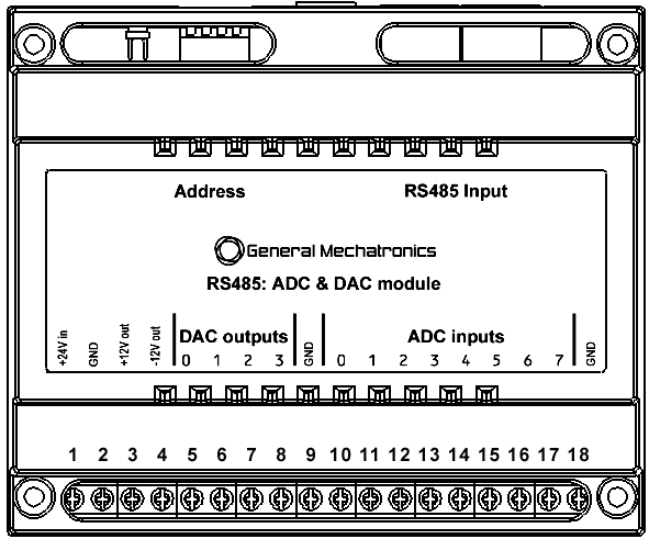
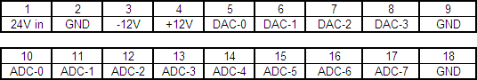
LinuxCNC HAL configuration
All the pins and parameters are updated by the following function:
gm.<nr. of card>.rs485
It should be added to the servo thread or other thread with larger period to avoid CPU overload.
Every RS485 module pin and parameter name begins as follows:
gm.<nr. of card>.rs485.<modul ID> ,where <modul ID> is from 00 to 15.
Pins:
.adc-<0-7>(float, Out)--Value of ADC input in Volts.
.dac-enable-<0-3>(bit, In)--Enable DAC output. When enable is false DAC
output is set to 0.0 V.
.dac-<0-3>(float, In) --Value of DAC output in Volts.
Parameters:
.adc-scale-<0-7>(float, R/W)--The input voltage will be multiplied by scale before being output to .adc- pin.
.adc-offset-<0-7>(float, R/W)--Offset is subtracted from the hardware input voltage after the scale multiplier has been applied.
.dac-offset-<0-3>(float, R/W)--Offset is added to the value before the hardware is updated.
.dac-high-limit-<0-3>(float, R/W)--Maximum output voltage of the hardware in volts.
.dac-low-limit-<0-3>(float, R/W)--Minimum output voltage of the hardware in volts.
For example:
gm.0.rs485.0.adc-0 – First analogue channel of the node.
gm.0 – Means the first PCI motion control card (PCI card address = 0).
.rs485.0 – Select node with address 0 on the RS485 bus.
.adc-0 – Select the first analogue input of the module.
13.5.4. Teach pendant module
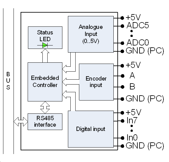
Electrical characteristics
Power:
Bus voltage:12V
Bus power consumption:100mA
Maximum load of 5V outputs:500mA
AD converter:
Input voltage range:0.5V
Input leakage current:50nA
Analogue input resistance:100MΩ
Input pin characteristics (Digital inputs and encoder inputs):
These are simple non-isolated I/O ports for general purpose usage. All voltage levels are referenced to the PC ground.
Absolute minimum input voltage:-0.5V
Absolute maximum input voltage:5.5V
Maximum low level input voltage:0.3V
Minimum high level input voltage:0.6V
Input leakage current1µA
Connection
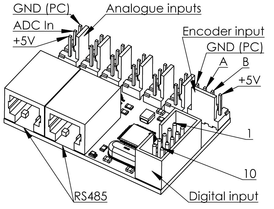
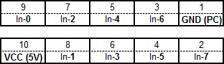
LinuxCNC HAL configuration
All the pins and parameters are updated by the following function:
gm.<nr. of card>.rs485
It should be added to the servo thread or other thread with larger period to avoid CPU overload.
Every RS485 module pin and parameter name begins as follows:
gm.<nr. of card>.rs485.<modul ID> ,where <modul ID> is from 00 to 15.
Pins:
.adc-<0-7>(float, Out)--Value of ADC input in Volts.
.dac-enable-<0-3>(bit, In)--Enable DAC output. When enable is false DAC
output is set to 0.0 V.
.dac-<0-3>(float, In) --Value of DAC output in Volts.
Parameters:
.adc-scale-<0-7>(float, R/W)--The input voltage will be multiplied by scale before being output to .adc- pin.
.adc-offset-<0-7>(float, R/W)--Offset is subtracted from the hardware input voltage after the scale multiplier has been applied.
.dac-offset-<0-3>(float, R/W)--Offset is added to the value before the hardware is updated.
.dac-high-limit-<0-3>(float, R/W)--Maximum output voltage of the hardware in volts.
.dac-low-limit-<0-3>(float, R/W)--Minimum output voltage of the hardware in volts.
For example:
gm.0.rs485.0.adc-0 – First analogue channel of the node.
gm.0 – Means the first PCI motion control card (PCI card address = 0)
.rs485.0 – Select node with address 0 on the RS485 bus
.adc-0 – Select the first analogue input of the module
13.5.5. Mechanical dimensions
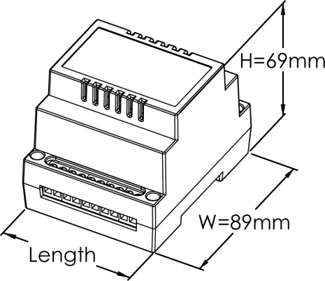
Lengths of each module:
Relay output module:139mm
Input module:65mm
ADC & DAC module:107mm
13.6. Digital Servo Drives (BMEGEMIMM25)
Homework
Select an industrial machine tool, for example CNC milling machine, CNC lathe or industrial robot. Review the corresponding literature (user’s guide, book of machine). Prepare the block diagram of the machine’s control and describe the operation of the block diagram. The project will be accepted only in the case that there are no theoretical mistakes in it. Two or three students may work on one project. In the case of three students in one project, the selected machine has to be more complex and it has to include an additional part (like tool magazine, cooling circuit, automatic door, etc.). Please consult with your instructor in the case of substantially different problem.
Signature: 7th week of lecture period, Submission deadline: 14th week of the lecture period
Students:
|
Name |
Neptun code |
Signature | |
|
1. | |||
|
2. | |||
|
3. |
Selected machine:
|
Type (eg.: SCARA robot-arm) |
Manufacturer (eg.: SEIKO) |
Model noumber (eg.: D-TRAN TT 4000 SC) |
Degree of freedom (eg.: 4) |
End-effector (eg.: megfogó) |
Task description (in the case of individual project):
…………………………………………………………………………………………………………………………………………………………………………………………………………………………………………………………………………………………………………………………………………………………………………………………………………
The project is (instructor fills it out)
issued by: Name: ………………………………..... Date: .……………………...
signed: Name: ………………………………..... Date: ………………………
approved: Name: ……………………………… Date: ………………………
Grade: …………..
13.7. Robot application Homework (Sample)
13.7.1. Authors
Zsolt Baranyai
Andor Szabolcs Simó
13.7.2. Project description
Understanding of the selected machine’s control. Displaying the control’s of the block diagram. Documenting the implementation of one selected part at wiring level.
13.7.3. Selected machine
The selected machine is PUMA 560 robot. The machine has 6 degrees of freedom. There are 6 revolute joints in the robot’s structure, where the last three represent a wrist. The joints are actuated by direct current. The positioning is solved by incremental encoders, which also have an index sign. Initializations of the absolute values are obtained by using an absolute potentiometer.
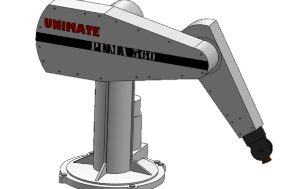
An universal gripper is chosen as the end effector of the robot. The end effector is driven by open and close logical commands. The robot brake function is also included into the model which stops the robot in case of any disturbance. This function is inegrated in the E-Stop circuit.
13.7.4. Elaboration in summary
The actuators, sensors, power amplifiers are kept the same as in original the original assembly. The analog servo is also kept thus the reference signal has to be the torque.
The communication is determined by the TTL on the side of the robot. While on the control’s side, the moduls are used for communication.
The idea is that all the additional parts are placed in a control cabinet, including the PC. Therefore common grounding can be used.
The designed block diagram is in the appendix. Where the break and the overheating events and their wiring are detailed in a schematic diagram.
The original control of the PUMA 560 is in the Figure 12-25, where the framed part is kept.
|
|
|
Figure 12-25. The original control of the PUMA 560. |
|
http://citeseerx.ist.psu.edu/viewdoc/summary?doi=10.1.1.56.815 download: 2013. november 2. Nuno Moreira et al [1996]: First Steps Towards an Open Control Architecture for a PUMA 560 |
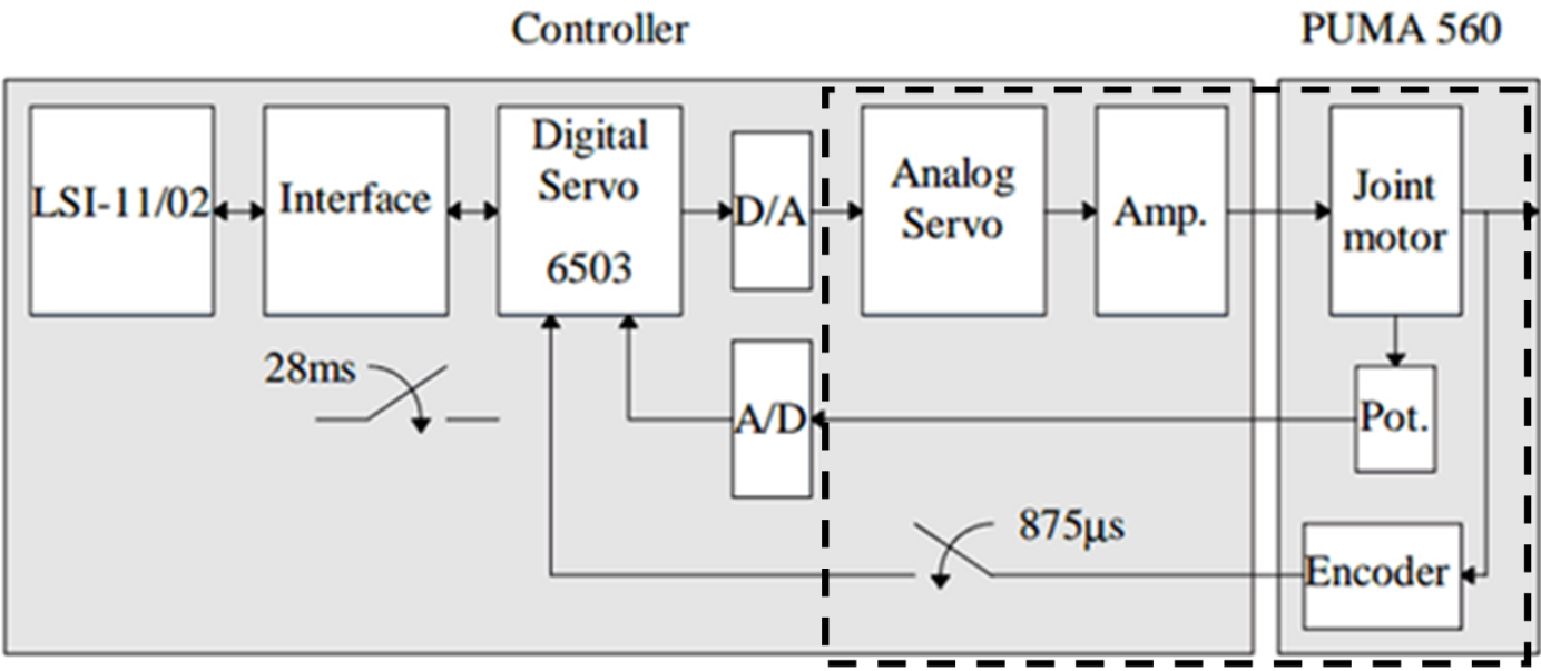
13.7.5. Attachment
Block diagram of the control.
Breakout and DAC modules.
Table of the robot’s wiring and control.
Connection of the Encoder breakout and the DAC modules. More details are presented in the attached table.
13.7.6. Blockdiagram of the control
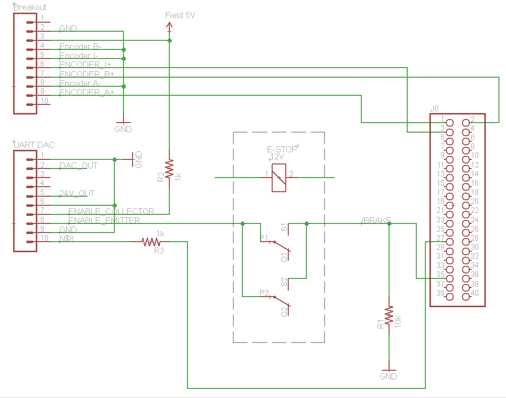
Breakout and DAC modules
|
Robot plugs | ||||||
|
J5 |
|
Place of the connection |
| |||
|
Pin |
Name |
Modul |
Pin |
Name |
Comment | |
|
1 |
POT_J1 |
|
RS485 ADC/DAC |
10 |
ADC-0 |
|
|
2 |
POT_J2 |
|
RS485 ADC/DAC |
11 |
ADC-1 |
|
|
3 |
POT_J3 |
|
RS485 ADC/DAC |
12 |
ADC-2 |
|
|
4 |
POT_J4 |
|
RS485 ADC/DAC |
13 |
ADC-3 |
|
|
5 |
POT_J5 |
|
RS485 ADC/DAC |
14 |
ADC-4 |
|
|
6 |
POT_J6 |
|
RS485 ADC/DAC |
15 |
ADC-5 |
|
|
7 |
POT_J7 |
|
|
NC |
|
|
|
8 |
POT_J8 |
|
|
NC |
|
|
|
9 |
ADGND |
|
|
GND |
GND |
|
|
10 |
AD+5V |
|
|
Field 5V |
Field 5V |
|
|
11 |
NC |
|
|
NC |
|
|
|
12 |
NC |
|
|
NC |
|
|
|
13 |
+12V |
|
RS485 ADC/DAC |
4 |
+12V |
|
|
14 |
+12V |
|
RS485 ADC/DAC |
4 |
+12V |
|
|
15 |
DAGND |
|
|
GND |
|
|
|
16 |
DAGND |
|
|
GND |
|
|
|
17 |
-12V |
|
RS485 ADC/DAC |
3 |
-12V |
|
|
18 |
-12V |
|
RS485 ADC/DAC |
3 |
-12V |
|
|
19 |
DAC+J1 |
|
UART/DAC 0 |
2 |
Analog out |
|
|
20 |
DAC-J1 |
|
|
GND |
GND |
|
|
21 |
DAC+J2 |
|
UART/DAC 1 |
2 |
Analog out |
|
|
22 |
DAC-J2 |
|
|
GND |
GND |
|
|
23 |
DAC+J3 |
|
UART/DAC 2 |
2 |
Analog out |
|
|
24 |
DAC-J3 |
|
|
GND |
GND |
|
|
25 |
DAC+J4 |
|
UART/DAC 3 |
2 |
Analog out |
|
|
26 |
DAC-J4 |
|
|
GND |
GND |
|
|
27 |
DAC+J5 |
|
UART/DAC 4 |
2 |
Analog out |
|
|
28 |
DAC-J5 |
|
|
GND |
GND |
|
|
29 |
DAC+J6 |
|
UART/DAC 5 |
2 |
Analog out |
|
|
30 |
DAC-J6 |
|
|
GND |
GND |
|
|
31 |
DAC+J7 |
|
|
GND |
GND |
|
|
32 |
DAC-J7 |
|
|
GND |
GND |
|
|
33 |
DAC+J8 |
|
|
GND |
GND |
|
|
34 |
DAC-J8 |
|
|
GND |
GND |
|
|
|
|
|
|
|
|
|
|
J6 |
|
|
|
|
| |
|
1 |
ENCA1 |
|
Breakout 0 |
9 |
Encoder A+ |
|
|
2 |
ENCB1 |
|
Breakout 0 |
7 |
Encoder B+ |
|
|
3 |
ENCI1 |
|
Breakout 0 |
6 |
Encoder I+ |
|
|
4 |
ENCA2 |
|
Breakout 1 |
9 |
Encoder A+ |
|
|
5 |
ENCB2 |
|
Breakout 1 |
7 |
Encoder B+ |
|
|
6 |
ENCI2 |
|
Breakout 1 |
6 |
Encoder I+ |
|
|
7 |
ENCA3 |
|
Breakout 2 |
9 |
Encoder A+ |
|
|
8 |
ENCB3 |
|
Breakout 2 |
7 |
Encoder B+ |
|
|
9 |
ENCI3 |
|
Breakout 2 |
6 |
Encoder I+ |
|
|
10 |
ENCA4 |
|
Breakout 3 |
9 |
Encoder A+ |
|
|
11 |
ENCB4 |
|
Breakout 3 |
7 |
Encoder B+ |
|
|
12 |
ENCI4 |
|
Breakout 3 |
6 |
Encoder I+ |
|
|
13 |
ENCA5 |
|
Breakout 4 |
9 |
Encoder A+ |
|
|
14 |
ENCB5 |
|
Breakout 4 |
7 |
Encoder B+ |
|
|
15 |
ENCI5 |
|
Breakout 4 |
6 |
Encoder I+ |
|
|
16 |
ENCA6 |
|
Breakout 5 |
9 |
Encoder A+ |
|
|
17 |
ENCB6 |
|
Breakout 5 |
7 |
Encoder B+ |
|
|
18 |
ENCI6 |
|
Breakout 5 |
6 |
Encoder I+ |
|
|
19 |
GND |
|
|
GND |
GND |
|
|
20 |
GND |
|
|
GND |
GND |
|
|
21 |
Vcc |
|
|
Field 5V |
Field 5V |
|
|
22 |
Vcc |
|
|
Field 5V |
Field 5V |
|
|
23 |
NC |
|
|
NC |
NC |
|
|
24 |
NC |
|
|
NC |
NC |
|
|
25 |
NC |
|
|
NC |
NC |
|
|
26 |
/STOP |
|
|
NC |
NC |
There is a separate E-Stop. |
|
27 |
THERM1 |
|
UART/DAC 0 |
10 |
Fault Anode |
1kOhm resistance |
|
28 |
THERM2 |
|
UART/DAC 1 |
10 |
Fault Anode |
1kOhm resistance |
|
29 |
THERM3 |
|
UART/DAC 2 |
10 |
Fault Anode |
1kOhm resistance |
|
30 |
THERM4 |
|
UART/DAC 3 |
10 |
Fault Anode |
1kOhm resistance |
|
31 |
THERM5 |
|
UART/DAC 4 |
10 |
Fault Anode |
1kOhm resistance |
|
32 |
THERM6 |
|
UART/DAC 5 |
10 |
Fault Anode |
1kOhm resistance |
|
33 |
NC |
|
|
NC |
NC |
|
|
34 |
NC |
|
|
NC |
NC |
|
|
35 |
/BRAKE |
|
E-Stop Relé |
2 |
E-Stop Relé |
NO |
|
36 |
HANDO |
|
RS-485 Relay |
1 |
0-NO |
|
|
37 |
HANDC |
|
RS-485 Relay |
4 |
1-NO |
|
|
38 |
UTIL4 |
|
|
NC |
NC |
|
|
39 |
UTIL5 |
|
|
NC |
NC |
|
|
40 |
UTIL6 |
|
|
NC |
NC |
|
13.7.7. Table: Connection of the robot and the control
|
Pin |
Signal |
Backplane |
Pin |
Signal |
Backplane | |
|
# |
Name |
Location |
# |
Name |
Location | |
|
1 |
POT_J1 |
J56A-F1 |
18 |
-12V |
TB5-4 | |
|
2 |
POT_J2 |
J56A-N1 |
19 |
DAC+J1 |
J103-11 | |
|
3 |
POT_J3 |
J56A-V1 |
20 |
DAC-J1 |
J103-12 | |
|
4 |
POT_J4 |
J56B-F1 |
21 |
DAC+J2 |
J103-13 | |
|
5 |
POT_J5 |
J56B-N1 |
22 |
DAC-J2 |
J103-14 | |
|
6 |
POT_J6 |
J56B-V1 |
23 |
DAC+J3 |
J103-15 | |
|
7 |
POT_J7 |
J56B-H2 |
24 |
DAC-J3 |
J103-16 | |
|
8 |
POT_J8 |
J56A-R2 |
25 |
DAC+J4 |
J103-17 | |
|
9 |
ADGND |
J56A-E2 |
26 |
DAC-J4 |
J103-18 | |
|
10 |
AD+5V |
J56A-F2 |
27 |
DAC+J5 |
J103-19 | |
|
11 |
NC |
28 |
DAC-J5 |
J103-20 | ||
|
12 |
NC |
29 |
DAC+J6 |
J103-21 | ||
|
13 |
+12V |
TB5-3 |
30 |
DAC-J6 |
J103-22 | |
|
14 |
+12V |
TB5-3 |
31 |
DAC+J7 |
J103-23 | |
|
15 |
DAGND |
TB5-2 |
32 |
DAC-J7 |
J103-24 | |
|
16 |
DAGND |
TB5-2 |
33 |
DAC+J8 |
J103-25 | |
|
17 |
-12V |
TB5-4 |
34 |
DAC-J8 |
J103-26 | |
|
1 |
ENCA1 |
J56A-A1 |
21 |
Vcc |
TB5-1 | |
|
2 |
ENCB1 |
J56A-C1 |
22 |
Vcc |
TB5-1 | |
|
3 |
ENCI1 |
J56A-E1 |
23 |
NC | ||
|
4 |
ENCA2 |
J56A-H1 |
24 |
NC | ||
|
5 |
ENCB2 |
J56A-K1 |
25 |
NC | ||
|
6 |
ENCI2 |
J56A-M1 |
26 |
/STOP |
J69-12c | |
|
7 |
ENCA3 |
J56A-P1 |
27 |
THERM1 |
J56A-B1 | |
|
8 |
ENCB3 |
J56A-S1 |
28 |
THERM2 |
J56A-J1 | |
|
9 |
ENCI3 |
J56A-U1 |
29 |
THERM3 |
J56A-R1 | |
|
10 |
ENCA4 |
J56B-A1 |
30 |
THERM4 |
J56B-B1 | |
|
11 |
ENCB4 |
J56B-C1 |
31 |
THERM5 |
J56B-J1 | |
|
12 |
ENCI4 |
J56B-E1 |
32 |
THERM6 |
J56B-R1 | |
|
13 |
ENCA5 |
J56B-H1 |
33 |
NC | ||
|
14 |
ENCB5 |
J56B-K1 |
34 |
NC | ||
|
15 |
ENCI5 |
J56B-M1 |
35 |
UTIL1 |
J103-5 |
/BRAKE |
|
16 |
ENCA6 |
J56B-P1 |
36 |
UTIL2 |
J44A-M2 |
HANDO |
|
17 |
ENCB6 |
J56B-S1 |
37 |
UTIL3 |
J44A-L2 |
HANDC |
|
18 |
ENCI6 |
J56B-U1 |
38 |
UTIL4 |
SPARE1 | |
|
19 |
GND |
TB5-2 |
39 |
UTIL5 |
SPARE2 | |
|
20 |
GND |
TB5-2 |
40 |
UTIL6 |
SPARE3 | |
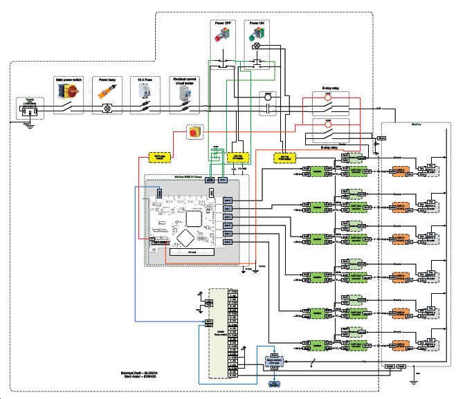
References
[1] Intelligent Robots and Systems, 2008. IROS 2008. IEEE/RSJ International Conference on. . OpenRDK: a modular framework for robotic software development. 2008.
[2] Az OpnRDK robot API, system official web page.
[3] YARP robot middleware official web page.
[4] OpenRTM-aist robot middleware official web page.
[5] Software deployment infrastructure for component based rt-systems. 3. 2011. Journal of Robotics and Mechatronics.
[6] Springer. Simulation, Modeling, and Programming for Autonomous Robots. . A software platform for component based rt-system development: Openrtm-aist. 2008.
[7] Intelligent Robots and Systems, 2005.(IROS 2005). 2005 IEEE/RSJ International Conference on. . RT-middleware: distributed component middleware for RT (robot technology). 2005. Intelligent Robots and Systems, 2005.(IROS 2005). 2005 IEEE/RSJ International Conference on.
[8] ROS (Robor Operating System) official web page.
[9] ICRA workshop on open source software. . ROS: an open-source Robot Operating System. 2009.
[10] A microprocessor-controlled speed regulator with instantaneous speed estimation for motor drives. 1. 95-99. Feb. 1988. IEEE Trans. Ind. Electron..
[11] 1st IFAC Congress. . Application of the theory of differential equations with discontinuous right-hand sides to non-linear problems in autimatic control. 923-925. 1960.
[12] Differential equations with discontinuous right-hand side. 199-231. 1964. Ann. Math Soc. Transl..
[13] Control Engineering. Red Business Information. Loop Tuning Fundamentals. July 1, 2003.
[14] Application of fully decoupled parity equation in fault detection and identification of dcmotors. 4. 1277-1284. June 2006. IEEE Trans. Ind. Electron..
[15] Determination of scaling factors for fuzzy logic control using the sliding-mode approach: Application to control of a dc machine drive. 1. 296-309. Feb. 2007. IEEE Trans. Ind. Electron..
[16] Energy-management system for a hybrid electric vehicle, using ultracapacitors and neural networks. 2. 614-623. Apr. 2006. IEEE Trans. Ind. Electron..
[17] Fuzzy controllers with maximum sensitivity for servosystems. 3. 1298-1310. Apr. 2007. IEEE Trans. Ind. Electron..
[18] Methods for constructing discountnuous planes in multidimensional variable structure systems. 10. 1466-1470. Oct. 1978. Automat. Remote Control.
[19] Sliding-mode control for high precision motion of a piezostage. 1. 629-637. Feb. 2007. IEEE Trans. Ind. Electron..
[20] Robust fuzzy neural network slidingmode control for two-axis motion control system. 4. 1209-1225. June 2006. IEEE Trans. Ind. Electron..
[21] Network-based fuzzy decentralized sliding-mode control for cat-like mobile robots. 1. 574-585. Feb. 2007. IEEE Trans. Ind. Electron..
[22] A high-performance sensorless indirect stator flux orientation control of industion motor drive. 1. 614-623. Feb. 2006. IEEE Trans. Ind. Electron..
[23] On Carath_Eodory's Conditions For The Initial Value Problem. 5. 1371{1376 S 0002-9939(97)03942-7 . 1997. Proceedings Of The American Mathematical Society.
[24] 1st IFAC Congr., pp. 923-925. Moscow . . Application of the Theory of Differential Equations with Discontinuous Right-hand Sides to Non-linear Problems in Automatic Control. 1960.
[25] Differential Equations with Discontinuous Right-hand Side. 199-231. 1964. Ann. Math Soc. Transl..
[26] 2nd Eur. Conf. On Power Electronics, Proc., pp 251-256. Grenoble . . Sliding Mode Control for Robotic Manipulators". 1987.
[27] EPE'91 4th European Conference on PowerElectronics, Proceedings vol. 3. pp. 3-180-184. Firenze . . Control of a Three Phase UPS Inverter with Unballanced and Nonlinear Load. 1991.
[28] Springer-Verlag. . Park Vector Based Sliding Mode Control K.D.Young, Ü. Özgüner (editors) Variable Structure System, Robust and Nonlinear Control.ISBN: 1-85233-197-6. 6. 1999. Springer-Verlag.
[29] Sliding Mode Design for Motion Control. 2000.
[30] Invariant Sliding Sector for Variable Structure Control. 2. 124-134. 2005. Asian Journal of Control.
[31] 8th Conference on Power Electronics and Motion Control Vol. 5, pp.5-254-5-259. . . Sector Sliding Mode Controller for Motion Control. 1998.
[32] Design of variable structure controllers with continuous switching control. 3. 409-431. 1996. INTERNATIONAL JOURNAL OF CONTROL.
[33] Variable Structure Control Optimization. 1992. Springer-Verlag.
[34] A Singular Perturbation Analysis of High-Gain Feedback Systems. 6. 931-938. 1977. IEEE Trans. on Automatic Control.
[35] Sliding Mode Control of a Discretee System. 145-152. 1990. System Control Letters.
[36] Sliding Mode in Dynamics Systems. 1029-1037. 1992. International Journal of Control.
[37] Controller Design for Manipulator using Theory of Variable Structure Systems. 101-109. 1978. IEEE Trans. on System, Man, and Cybernetics.
[38] Microprocessor Based Robot Manipulator Control with Sliding Mode". 1. 11-18. 1987. IEEE Trans. On Industrial Electronics.
[39] Application of Sliding Modes to Induction Motor. 1. 4149. 1981. IEEE Trans. On Industrial Appl..
[40] EDIS – Publishing Centre of Zilina University, ISBN 80-8070-087-7. Zilina . Forced Dynamics Control of Electric Drive. 2003.
[41] Sliding modes applications in power electronics and motion control systems. TU22 - TU31. 1999. Proceedings of the IEEE International Symposium Industrial Electronics.
[42] The 29th Annual Conference of the IEEE Industrial Electronics Society, IECON '03, Vol. 1, Page(s):997 - 1002. . Sliding modes in power electronics and motion control systems. 2003.
[43] 37th IEEE Power Electronics Specialists Conference, PESC '06. Page(s):1 - 7. . An Evaluation of the Practicality of Sliding Mode Controllers in DC-DC Converters and Their General Design Issues. 2006.
[44] Sliding Controller Design for Non-Linear Systems. 2. 421-434. 1984. Int. Journal of Control.
[45] The Third Worksop on Variable Structure Systems and Lyaponov Design . Napoly, Italy . Chattering Free Sliding Modes. 1994.
[46] Direct Torsion Control of Flexible Shaft based on an Observer Based Discrete-time Sliding Mode. 2. 291-296. 1998. IEEE Trans. on Industrial Electronics.
[47] L Frequency Domain Input–Output Analysis of Sliding-Mode Observers. 11. 1798-1803. 2006. IEEE Transactions on Automatic Control.
[48] Sliding-mode MRAS speed estimators for sensorless vector control of induction Machine. 1. 146 – 153 . 2005. IEEE Transactions on Industrial Electronics.
[49] Variable structure control with sliding sector. 211-228. 2000. Automatica.
[50] VS-control with time-varying sliding sector - Design and application to pendulum. 3. 307-316. 2004. ASIAN JOURNAL OF CONTROL.
[51] Tensor Product Model Transformation-based Sliding Surface Design. 4. 23-36. 2006. Acta Polytechnica Hungarica.
[52] The Chattering Analysis. 2006. EPE-PEMC Proceedings 36.
[53] Robust frequency shaping sliding mode control” Control Theory and Applications. 3. 312 – 320. 2000. IEE Proceedings.
[54] ‘Sliding surface design in thefrequency domain’, in ‘Variable Structure and Lyapunov control’,ZINOBER, A.S.I. (Ed.) (), . 75-84. 1994. Springer-Verlag, Berlin.
[55] Proceedings of the 39th IEEE Conference on Decision and Control, pp. 4765 – 4770. . Adaptive backstepping control of nonlinear systems with unmatched uncertainty. 2000 .
[56] The fusion of computationally intelligent methodologies and sliding-mode control-A survey. 1. 4 – 17. 2001. IEEE Transactions on Industrial Electronics.
[57] H Robust Fuzzy Neural Network Sliding-Mode Control for Two. 4. 1209 – 1225 . 2006. Axis Motion Control System IEEE Transactions on Industrial Electronics.