Highly Automated Vehicle Systems
Copyright © 2014 Dr. Gáspár Péter, Dr. Szalay Zsolt, Aradi Szilárd

A tananyag a TÁMOP-4.1.2.A/1-11/1-2011-0042 azonosító számú „ Mechatronikai mérnök MSc tananyagfejlesztés ” projekt keretében készült. A tananyagfejlesztés az Európai Unió támogatásával és az Európai Szociális Alap társfinanszírozásával valósult meg.

Published by: BME MOGI
Editor by: BME MOGI
ISBN 978-963-313-173-2
2014
- 1. Control design aspects of highly automated vehicles
- 2. Layers of integrated vehicle control
- 3. Environment Sensing (Perception) Layer
- 4. Human-Machine Interface
- 5. Trajectory planning layer
- 6. Trajectory execution layer
- 7. Intelligent actuators
- 8. Vehicle to Vehicle interactions (V2V)
- 9. Vehicle to Infrastructure interaction (V2I)
- 10. Vehicle to Environment interactions (V2E)
- 11. Different methods for platooning control
- 12. Vehicle control considering road conditions
- 13. Design of decentralized supervisory control
- 14. Fleet Management Systems
- 15. References
- References
- 1.1. Road fatalities in the EU since 2001 (Source: CARE)
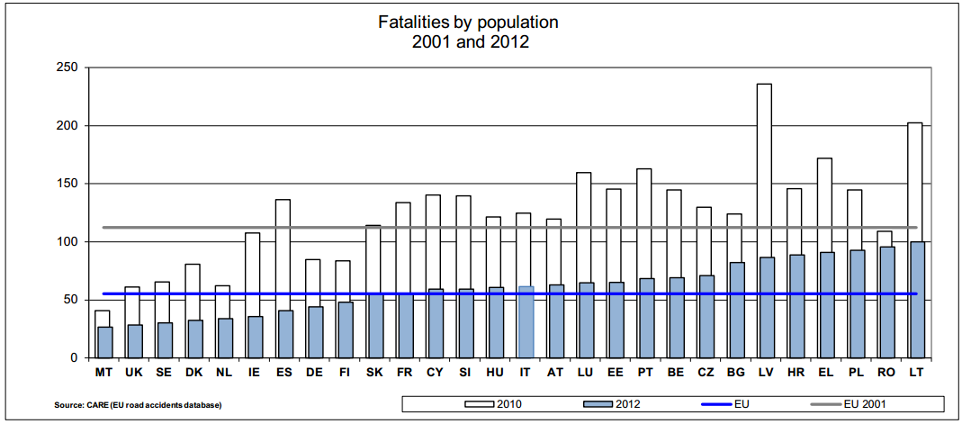
- 1.2. Road fatalities by population since 2001 (Source: CARE)
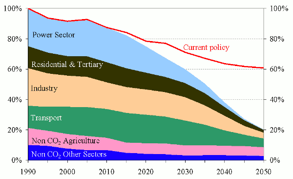
- 1.3. European roadmap for moving to a low-carbon economy (Source: EU)
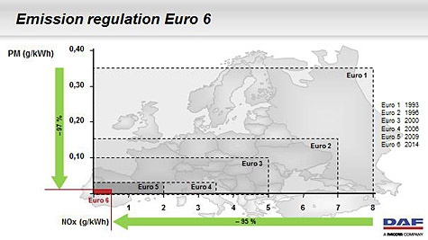
- 1.4. European Euro 6 emissions legislation (Source: DAF)
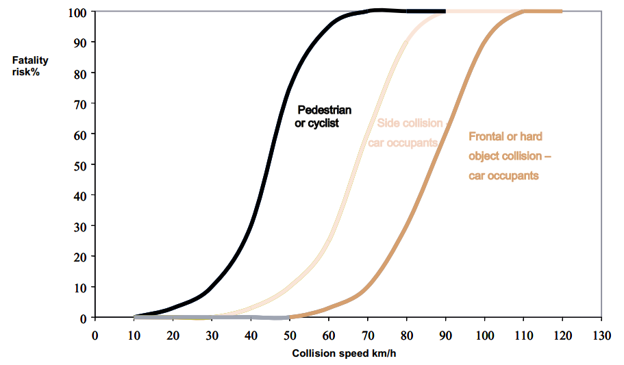
- 1.5. The effect of collision speed on fatality risk (Source: UNECE)
- 1.6. Situations when driver assistance is required. (Source: HAVEit)
- 1.7. Automation level approach by the HAVEit system. (Source: HAVEit)
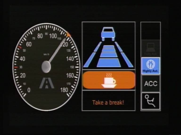
- 1.8. Driver drowsiness warning: Time to take a coffee break! (Source: HAVEit)
- 1.9. LDW support guiding the driver back into the centre of the lane. (Source: Mercedes-Benz)
- 1.10. Counter-steering torque provided to support keeping the lane. (Source: TRW)
- 1.11. Warning for misuse of lane assist for autonomous driving. (Source: Audi)
- 1.12. Parking space measurement (Source: Bosch)
- 1.13. Principle of the operation of the parking aid systems (Source: Bosch)
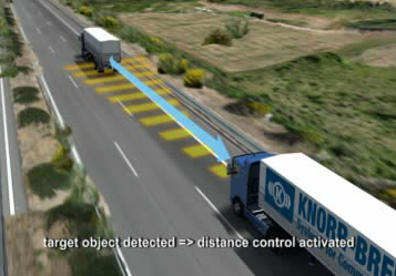
- 1.14. ACC distance control function for commercial vehicles (Source: Knorr-Bremse)
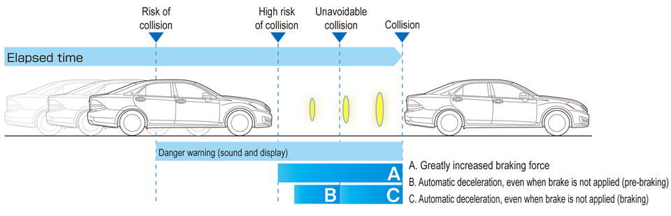
- 1.15. Steps of collision mitigation with an ACC System (Source: Toyota)
- 1.16. Temporary Auto Pilot in action at 130 km/h speed (Source: Volkswagen)
- 1.17. Highly automated driving on motorways (Source: BMW)
- 1.18. Test vehicle with automated highway driving assist function (Source: Toyota)
- 1.19. Demonstrating automated roadwork assistance functionality. (Source: HAVEit)
- 1.20. Demonstration of a platoon control
- 1.21. Hierarchical structure applied in the PATH project
- 1.22. Google’s self-driving test car, a modified hybrid Toyota Prius (Source: http://www.motortrend.com)
- 2.1. Levels of intelligent vehicle control (Source: Prof. Palkovics)
- 2.2. Initial model of the HAVEit architecture simulation
- 2.3. Levels of intelligent vehicle control (Source: PEIT)
- 2.4. HAVEit System Architecture and Layer structure (Source: HAVEit)
- 2.5. Powertrain Control Structure of the execution layer (Source: PEIT)
- 2.6. Scheme of the integrated control
- 2.7. Reference control architecture for autonomous vehicles (NIST)
- 3.1. Sensor devices around the vehicle (Source: Prof. Dr. G. Spiegelberg)
- 3.2. Radar-based vehicle functions (Source SaberTek)
- 3.3. Principle of FM-CW radars (Source: Fujitsu-Ten)
- 3.4. Frequency allocation of 77 GHz band automotive radar
- 3.5. Bosch radar generations (Source: Bosch)
- 3.6. Measurement principle of ultrasonic sensor
- 3.7. The emitted and echo pulses (Source: Banner Engineering)
- 3.8. Bosch ultrasonic sensor (Source: Bosch)
- 3.9. Ultrasonic sensor system (Source: Cypress)
- 3.10. Structure of CCD (Source: Photonics Spectra)
- 3.11. Structure of CMOS sensor (Source: Photonics Spectra)
- 3.12. Principle of colour imaging with Bayer filter mosaic (Source: http://en.wikipedia.org/wiki/File:Bayer_pattern_on_sensor_profile.svg)
- 3.13. Bosch Multi Purpose Camera (Source: http://www.bosch-automotivetechnology.com/)
- 3.14. Bosch Stereo Video Camera (Source: http://www.bosch-automotivetechnology.com/)
- 3.15. Passive thermal image sensor (source: http://www.nature.com, BMW))
- 3.16. Night vision system display (source: BMW)
- 3.17. Typical laser scanner fusion system installation with 3 sensors. (Source: HAVEit)
- 3.18. :The laser scanner sensor itself and its installation point front left below the beams. (Source: HAVEit)
- 3.19. Multi-layer technology enables pitch compensation and lane detection. (Source: HAVEit)
- 3.20. Velodyne HDL-64E laser scanner (Source: Velodyne)
- 3.21. General architecture of laser scanners (Source: Velodyne)
- 3.22. Laser scanner fusion with 360 degrees scanning. (Source: IBEO)
- 3.23. Image of a point cloud from a laser scanner (Source: Autonomous Car Technology)
- 3.24. Position calculation method based on 3 satellite data. (Source: http://www.e-education.psu.edu)
- 3.25. Long March rocket head for launching Compass G4 satellite (Source: http://www.beidou.gov.cn)
- 3.26. BeiDou 2nd Deployment Step(Source: http://gpsworld.com/the-system-vistas-from-the-summit/)
- 3.27. Comparison of BeiDou with GPS(Source: http://gpsworld.com/china-releases-public-service-performance-standard-for-beidou/)
- 3.28. Differential GPS operation (source: http://www.nuvation.com)
- 3.29. Environment sensor positions on the HAVEit demonstrator vehicle. (Source HAVEit)
- 3.30. Block diagram of a sensor data fusion system: inputs and outputs. (Source HAVEit)
- 4.1. Example for the congested and confusing HMI (Source: Knight Rider series)
- 4.2. The vision of project AIDE (Source: AIDE)
- 4.3. HMI design: AQuA, take over request. (Source: HAVEit)
- 4.4. BMW iDrive controller knob (Source: BMW)
- 4.5. Splitview technology of an S-Class vehicle (Source: Mercedez-Benz)
- 4.6. Indicator stalk with cruise control and light switches (Source: http://www.carthrottle.com/)
- 4.7. Integrated radio and HVAC control panel with integrated knobs (Source: TRW)
- 4.8. Resistive touchscreen (Source: http://www.tci.de)
- 4.9. Projected capacitive touchscreen (Source: http://www.embedded.de)
- 4.10. Old instrument cluster: electronic gauges, LCD, control lamps (Source: BMW)
- 4.11. Liquid crystal display operating principles (Source: http://www.pctechguide.com)
- 4.12. A flexible OLED display prototype (Source: http://www.oled-info.com)
- 4.13. The SPORT+ and COMFORT modes of the BMW 5 Series’ instrument cluster (Source: http://www.bmwblog.com)
- 4.14. The SPORT+ and COMFORT modes of the BMW 5 Series’ instrument cluster (Source: http://www.bmwblog.com)
- 4.15. Head-Up Display on the M-Technik BMW M6 sports car. (Source. BMW)
- 4.16. Next generation HUD demonstration (Source: GM)
- 4.17. Excerpt from the ECE Regulations (Source: UNECE)
- 4.18. Combination of driver state assessment (Source: HAVEit)
- 5.1. Speed and distance profile comparison of standard ACC versus Cooperative ACC systems (Source: Toyota)
- 5.2. Illustration of the parallel parking trajectory segmentation (Source: Ford)
- 5.3. Layout of common parking scenarios for automated parking systems (Source: TU Wien)
- 5.4. Traffic jam assistant system in action (Source: Audi)
- 5.5. The operation of today’s Lane Keeping Assist (LKA) system (Source: Volkswagen)
- 5.6. Automated Highway Driving Assist system operation (Source: Toyota)
- 5.7. Scenarios of single or combined longitudinal and lateral control (Source: Nissan)
- 5.8. The manoeuvre grid with priority rankings (Source: HAVEit)
- 5.9. The decision of the optimum trajectory (Source: HAVEit)
- 6.1. Division of road
- 6.2. Simplified vehicle model
- 6.3. Implementation of the controlled system
- 6.4. Architecture of the low-level controller
- 6.5. Architecture of the control system
- 6.6. Counterbalancing side forces in cornering maneuver
- 6.7. Relationship between supply and demand of side friction in a curve
- 6.8. Relationship between curve radius and safe cornering velocity
- 6.9. The arc of the vehicle path
- 6.10. Validation of the calculation method
- 7.1. Intelligent actuators influencing vehicle dynamics (Source: Prof. Palkovics)
- 7.2. The role of communication networks in motion control (Source: Prof. Spiegelberg)
- 7.3. CAN bus structure (Source: ISO 11898-2)
- 7.4. Categorization of failure during risk analysis (Source: EJJT5.1Tóth)
- 7.5. Characterization of functional dependability (Source: EJJT5.1 Tóth)
- 7.6. Redundant energy management architecture (Source: PEIT)
- 7.7. Electronic power assisted steering system (TRW)
- 7.8. Superimposed steering actuator with planetary gear and electro motor (ZF)
- 7.9. Steer-by-wire actuator installed in the PEIT demonstrator (Source: PEIT)
- 7.10. Safety architecture of a steer-by-wire system (Source: HAVEit)
- 7.11. Direct Adaptive Steering (SbW) technology of Infiniti (Source: Nissan)
- 7.12. Retrofit throttle-by-wire (E-Gas) system for heavy duty commercial vehicles (Source: VDO)
- 7.13. Layout of an electronically controlled braking system (Source: Prof. von Glasner)
- 7.14. Layout of an Electro Pneumatic Braking System (Source: Prof. Palkovics)
- 7.15. Layout of an Electro Hydraulic Braking System (Source: Prof. von Glasner)
- 7.16. Layout of an Electro Mechanic Brake System (Source: Prof. von Glasner)
- 7.17. Clutch-by-wire system integrated into an AMT system (Source: Citroen)
- 7.18. Schematic diagram of an Automated Manual Transmission (Source: ZF)
- 7.19. Layout of a dual clutch transmission system (Source: howstuffworks.com)
- 7.20. Cross sectional diagram of a hydrodynamic torque converter with planetary gear (Source: Voith)
- 7.21. CVT operation at high-speed and low-speed (Source: Nissan)
- 8.1. V2V interactions (Source: http://www.kapsch.net)
- 8.2. Infrastructure-based and Ad hoc networks example (Source: http://www.tldp.org)
- 8.3. Vehicular Ad Hoc Network, VANET (source: http://car-to-car.org)
- 8.4. Multi-hop routing (Source: http://sar.informatik.hu-berlin.de)
- 8.5. Multicast communication (Source: http://en.wikipedia.org/wiki/File:Multicast.svg)
- 8.6. Bogus information attack
- 8.7. V2V standards and communication stacks (Source: Jiang, D. and Delgrossi, L.)
- 8.8. DSRC spectrum band and channels in the U.S.
- 8.9. DSRC spectrum allocation worldwide
- 8.10. V2V application examples (forrás:http://gsi.nist.gov/global/docs/sit/2010/its/GConoverFriday.pdf)
- 8.11. Hazardous location warning (source: http://car-to-car.org)
- 8.12. Privileging fire truck (source: http://car-to-car.org)
- 8.13. Reporting accidents (source: http://car-to-car.org)
- 8.14. Intelligent intersection (source: http://car-to-car.org)
- 8.15. V2V based Cooperative-adaptive Cruise Control test vehicle. (Source: Toyota)
- 9.1. Architecture example of V2I systems. (Source: ITS Joint Program Office, USDOT)
- 9.2. Collisions avoided using Adaptive Frequency Hopping
- 9.3. Example safety applications with the integration of DSRC and roadside sensors (Source: http://www.toyota-global.com)
- 9.4. Dynamic traffic control supported by DSRC (Source: http://www.car-to-car.org/)
- 10.1. Combined pedestrian detection (Source: http://www.roadtraffic-technology.com, AGD Systems)
- 10.2. Loop detector after installation (Source: http://www.fhwa.dot.gov/publications/publicroads/12janfeb/05.cfm)
- 10.3. Highway toll control cameras (Source: www.nol.hu)
- 10.4. Portable speed warning sign at city entrance. (Source: http://www.telenit.hu)
- 10.5. Radar-based measurement solution (Source: http://www.roadtraffic-technology.com, AGD Systems)
- 11.1. Illustration of a platoon in the CarSim software
- 11.2. Structure of a platoon system
- 11.3. Illustration of a platoon
- 11.4. Mini-platoon information structure
- 12.1. The effects of the forward velocity to the suspension system
- 12.2. The effects of the road roughness to the suspension system when the velocity is
- 13.1. The supervisory decentralized architecture of integrated control
- 14.1. System structure
- 14.2. General architecture of the on-board unit
- 14.3. Architecture of the central system
- 14.4. Diagram example
- 14.5. Example alarm log
- 14.6. Vehicle parameters’ statistics example
- 14.7. Journey log example
- 14.8. Vector map example
- 14.9. Google Maps based FMS example
Chapter 1. Control design aspects of highly automated vehicles
In the following pages the authors would like to provide an introduction into the design, the architecture and functionality of today’s highly automated vehicle control systems. Thanks to the developments in electronics technology integrated into the automotive industry there has been a revolution in road vehicle technology in the past 20 years. In modern vehicles there are approximately 100 microcomputers today providing service to the driver by means of vehicle operation, comfort, assistance and safety. Electronics control almost every function inside the vehicle and there are attempts to harmonise vehicle-to-vehicle communication (V2V) and vehicle-to-infrastructure information exchange (V2I) as well. Advanced driver assistance systems (ADAS) take over more and more complex and complicated tasks from the driver like adaptive cruise control (ACC) or lane keeping assistance (LKA), to make driving even easier and safer. In the not too far future the public road vehicles will be able to drive without a driver. On one hand the technology improvements makes such functions feasible even on public roads, while on the other hand it raises new challenges to policy makers. Until that time there are a lot of tasks to be solved, several technical questions and maybe even more legal issues have to be answered.
1.1. Motivation
1.1.1. Reducing accident number and accident severity
Reducing the number of accidents and accident severity is the highest importance according to the EU objectives, but this in not only a European, but a global problem affecting the whole society. Worldwide every year almost 50 million people are injured and 1.2 million people die in road accidents; more than half of them being young adults aged 15 to 44. Forecasts indicate that, without substantial improvements in road safety, road accidents will be the second largest cause of healthy life years lost by 2030. (Source:[1])
In Europe there is no reality to further improve the currently existing road network, so the solution has to face the limited infrastructure and the even further growing demand of transport. That is why highly automated road vehicles (integrated into an intelligent environment) will have a key role in improving road safety. The EU road safety strategy defined in 2001 has achieved significant results, but there is still a lot to do. The following figures [2] below show the overall and country based progress achieved in saving lives on European roads.
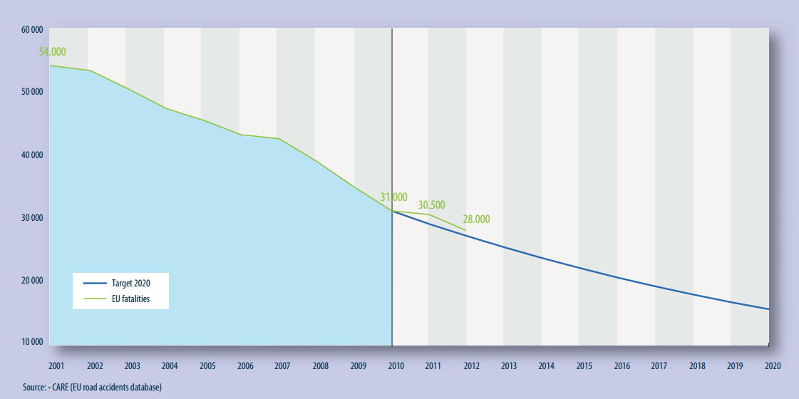
Hungary has been recognised with the “2012 Road Safety PIN Award” at the 6th ETSC Road Safety PIN Conference in 2012 for the outstanding progress made in reducing road deaths. Road deaths in Hungary have been cut by 49% since 2001, helped by a 14% decrease between 2010 and 2011. Since 2004 and its accession to the EU, Hungary quickly adapted to the rigours of membership and to the challenge of the EU 2010 target. (Source: [3])
1.1.2. Saving energy and reducing harmful exhaust emission
The other global challenge is to make transportation more efficient and environment friendly. Europe accelerates its progress towards a low-carbon society in order to reach the target of an 80% reduction in emissions below the 1990 levels by 2050. To be able to achieve that, the emissions should be reduced 40% by 2030 and 60% by 2040. Each sector has to contribute to achieve this, and transportation has an essential part in that. (Source: [4])
Although more economical engines (see also downsizing technology) also results in less emission, on the other hand there has been a great improvement recently in exhaust gas handling technology thanks to the EU regulations. Since the introduction of the Euro1 standard (1993) the harmful exhaust emission level was reduced the limit for NOX by 95% and for particulates by 97% to the Euro 6 levels. Figure 4 shows European harmful exhaust emission reduction requirements. (Source: [5])
Highly automated driving has also a value add to efficiency and lower harmful emissions by functions like Active Green Driving (AGD), Automated Queue Assistance (AQUA), forward thinking driving with eHorizon and velocity profile planning.
The main goal of the Active Green Driving is to reduce the fuel consumption and potentially emissions in vehicles by using e-Horizon system enhanced with environment sensors and the continuous prediction of vehicle speed profile. This includes a fuel optimal powertrain strategy and a driver support interface to give driving recommendations, in certain defined situations, using both graphical and textual information and furthermore haptic feedback in the accelerator pedal. (Source:[6])
1.1.3. The role of mechatronics
One should understand that there are some objective factors that electronics (mechatronics) has no alternative in the future of driving. We should not forget that most of the drivers on public road are not professional pilots, but even the most talented driver cannot compete with intelligent mechatronic systems in the following fields:
limited information: the driver does not have access to the information that state-of-the–art sensors installed in every part of the vehicle provide. The precise and detailed information about the vehicle status and the surrounding environment is essential for decision making.(Perception layer)
limited time: information in electronic systems propagate with the speed of light. The reaction times of mechatronic systems are significantly shorter compared to any human or mechanic systems. Information exchange between intelligent electronics inside the vehicle network is comparable to business computer networks.
limited access: for example mechatronic systems can individually brake each and every wheel according to the circumstances that may change hundred times a second while the driver has only the possibility to press more or less the brake pedal.
The electronically networked driver assistance systems will have key factor in the increase of safety on roads. According to statistics only 3% of traffic accidents can be traced back to technical reasons (vehicle), while 97% of accidents are caused by human factors (driver). Beside the inadequate technical status of a certain vehicle, the major sources of vehicle accidents are wrong driver decision, inappropriate evaluation of the circumstances, or lack of consideration. The probability of wrong decisions radically increases if the driver is in bad physical or mental condition, for example tired or from some other kind of reason indisposed.
According to European accident statistics 2/3 of the accidents with serious outcome could have been avoidable by the usage of driver assistance systems. A considerable part of these accidents are pile-up accidents, from which more than half can be traced back to lack of attention. Beyond the pile-up, accidents where commercial vehicles are involved are typically caused by drifting out, jack-knifing or rolling over.
In case of losing vehicle stability, unintentional lane departure, pile-up happening from behind, there are technical solutions to warn the driver before a late recognition and - if it is not enough - assistance systems automatically intervene in the management of the vehicle, with which the consequences of the accident can be radically mitigated. Such intervention may be a last minute emergency braking, which may significantly reduce the kinetic energy of the vehicle before the collision. Driver assistance systems may also compensate for eventual erroneous reactions of the driver.
1.2. Design aspects
It is no question that highly automated driving will play a major role in personal mobility in the future. The question is only when and how. Highly automated driving systems will relieve the drivers from distracting or stressing tasks ensuring safer and sustainable mobility. Today’s road vehicles are already complicated enough to distract some driver segments from using new driver assistance features. User acceptance is a key figure in moving towards highly automated driving, since most of the drivers can benefit from automated assistance systems in special situations. The application should be very easy and seamless to promote such functions and new ADAS features must be introduced into the education of drivers to understand them and get used to them.
There are traffic circumstances when drivers are especially in need of assistance like driver overload or underload situations. Driver overload situation may occur when the driver has to carry out multiple tasks simultaneously while also having to pay attention to other vehicles (e.g. intensive situations like turning manoeuvres at intersections or driving in the narrow lanes of roadwork areas) and driver stress may result in a deteriorated performance. Driver underload situation occurs during monotonous driving when there are really few impulses reaching the driver resulting in drowsiness (e.g. boring situations like traffic jams or long distance driving). Under “normal” conditions the driver has enough driving activity to make him awake and focused while not too much to distract or confuse him, this can also be regarded as optimum driving fun.
Either driver underload or overload situation results in the degradation of driver performance that is a risk for the traffic environment. Highly automated driving is a promising way to reduce this risk by providing assistance to the driver in these special situations. The following figure shows the correlation between driver load and driver performance indicating the need for assistance.
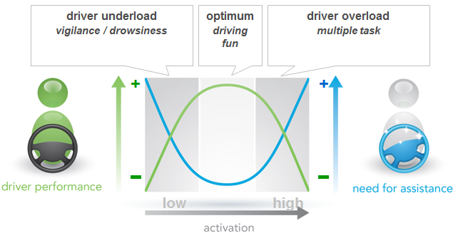
The two extreme situations on the figure above are not preferred. The resolution is selective automation of the vehicle, where the driver is still always a part of the control loop. (This is not just a requirement of legal issues but also important from user acceptance point of view.) In this approach the driver can pass over the control to the vehicle under specified circumstances and the vehicle can also pass back the control to the driver if the system is not able to handle the situation. Meanwhile the driver attention is continuously monitored and in case the driver is not capable of handling the traffic situation (e.g. medical emergency) the vehicle automatically takes over control and gradually reducing the vehicle speed safely drives to standstill on the roadside. The system will also pass back control to the driver if the pre-conditions for highly automated driving are not met, e.g. if no lane markings can be detected.
1.3. Automation levels
State-of-the-art driver assistant systems (ADAS) already provide a range of support functions for the driver. The vehicle automation level can be categorized into several layers depending on the degree of substituting driver tasks.
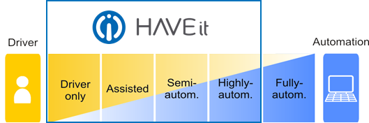
Based on the perception layer information the command layer determines the availability of each and every automation level in a hierarchical way. The availability may vary during driving according to the changing of the environment (e.g. lane markings obtainable or not). The automation levels may only change in order either upwards and downwards. Upon availability the driver is responsible for the selection of one of the automation levels. The driver cannot select an automation level that is not offered because the pre-conditions are not met. Vica versa if a certain automation level is no longer available the vehicle warns the driver to take over the control of the vehicle.
There are assistance levels that are built on each-other, assuming that the next level is available only in case all the previous levels are fulfilled.
1.3.1. Warning
The very first level of providing assistance to the driver is to inform the driver about potentially dangerous situations. In this stage there is no further support or intervention, the driver is just warned about the potential danger. The warning information is transmitted to the driver via the primary human machine interface (HMI) of the vehicle, using either visible (e.g. dashboard), acoustic (e.g. alarm sound) or haptic (e.g. seat or steering wheel vibration) feedback. It is totally up to the driver if he takes actions or not after receiving the warning. A good example is driver drowsiness detection which warns the driver to take a coffee break in case of fatigue by continuously monitoring the steering wheel movement. The warning message is an icon of a coffee cup in front of an orange background and there is a text message ”please take a break” shown in the figure below on the display of the HAVEit HMI.
1.3.2. Support
The second level of providing assistance is not just to warn the driver but support him guiding how to drive the car in a potentially hazardous situation. This level assumes that the driver is aware of the probably unsafe situation (warning) and there are hints provided further more to the driver directing him to the right manoeuvre.
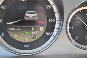
Lane Departure Warning is a basic function inside supported control. It warns the driver if he gets too close to the lane markings and then warns the driver by acoustic and visual warnings or a slight vibration in the steering wheel.
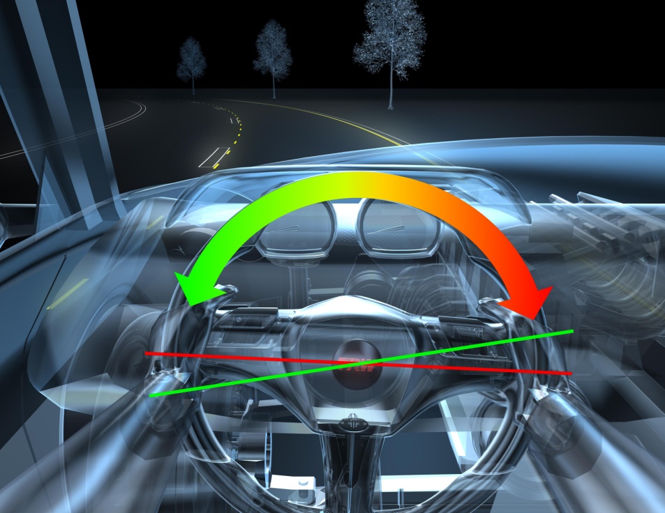
Additional support may also be providing a counter-steering torque with the electrically power assisted steering system (EPAS or EPS). The gently applied EPAS steering torque makes it harder to steer out (change lane without using the turn signal). The driver may still decide to change lane (without using the turn signal) and steer out from the lane by a stronger steering wheel movement or stay in the lane by gently steering back.
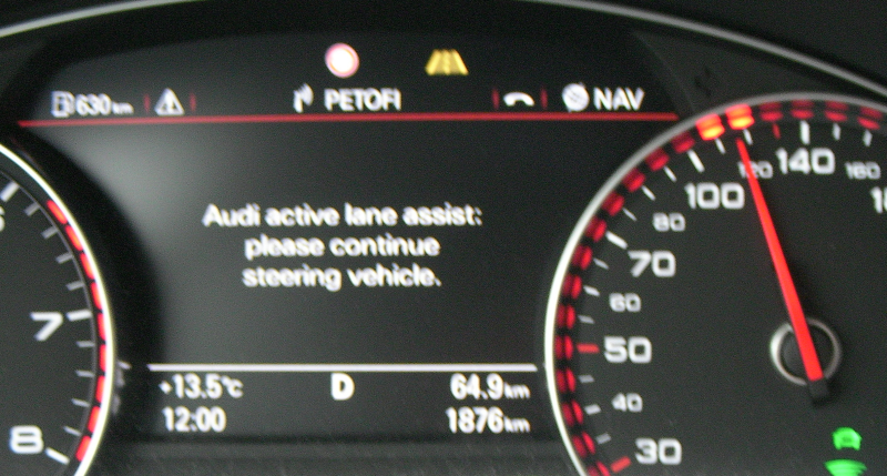
The function works camera based by analysing the lane markings on the road in front and by comparing the current vehicle direction in relation to them. It usually incorporates hands-off detection of the steering wheel to avoid the use (misuse) of the system for autonomous driving.
Another not safety but typical comfort function example is the parking assistant system which can cover the support level and furthermore the intervention level. Into the support level three functions can be enrolled: parking space measurement, parking aid information and park steering information.
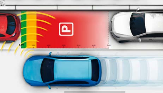
The parking aid information system monitors the close-up area in front and/or behind the vehicle by the ultrasonic sensors and informs the driver with an optical and/or acoustical signal of how close the vehicle is to an obstacle.
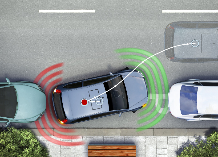
When the parking space measurement is active the ultrasonic sensors are scanning the roadside. As soon as the system identifies a suitable parking space long enough for the car, the driver will be immediately informed. The driver can activate the parking assistant with a push of button and initiate the parking manoeuvre.
The park steering information system provides clear instructions on steering-wheel position and the necessary stop and switching points through a display, thus guiding the driver into the perfect parking position.
1.3.3. Intervention
The next level of driver assistance is the automated intervention into the vehicle control. Depending on the intervention scale there are categories of semi-automated driving and highly automated driving. While during semi-automated driving the vehicle’s longitudinal movement is under automated control, as during highly automated driving both longitudinal and lateral control takes part of the vehicle motion.
1.3.3.1. Semi-automated intervention
Basically semi-automated driving can be described as supported driving plus longitudinal control of vehicle movement. The market currently offers several functions in this segment like adaptive cruise control (ACC) with Stop & Go extension or Emergency Brake Assist. This function uses a radar sensor to monitor the traffic ahead adjusting vehicle speed and keeping safe distance to the vehicle in front via the throttle-by-wire and brake-by-wire intelligent actuators. While no front vehicle is detected speed control is active keeping constant vehicle speed regardless of the road inclination, but when a vehicle is detected ahead then distance control becomes active, keeping speed-dependant safe distance between the two vehicles. The following figure shows the moment when distance control becomes active.
On top of ACC function there may be a collision avoidance (mitigation) option. Based on the radar signal (and video sensors), the system warns the driver if there is a collision hazard, and in case the collision is inevitable for the driver the system automatically applies the brakes to reduce vehicle speed, thus collision severity. Such function physically mitigates the collision consequences by reducing collision speed.
1.3.3.2. Highly automated intervention
The former levels of automated driving all had operational examples on the market, whereas highly-automated driving represents the state-of-the-art of road vehicle automation that soon (2016-2020) will be introduced to the public domain with function like Temporary Auto Pilot, Automated support for Roadwork and Congestion.
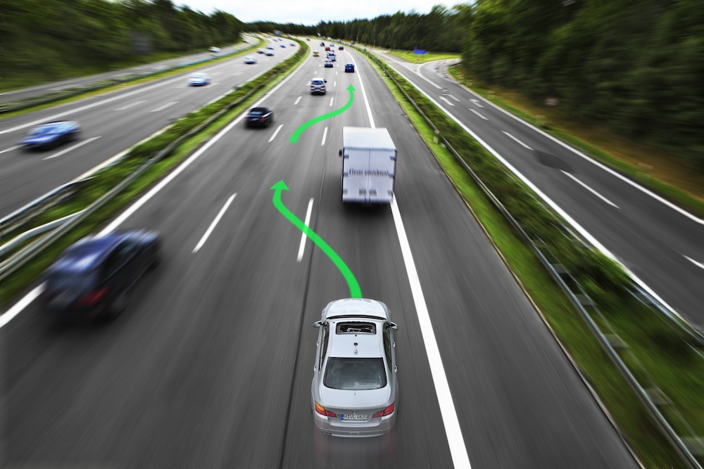
High automation means integrated longitudinal and lateral control of the vehicle enabling not only acceleration and braking for the vehicle automatically, but also changing lane and overtaking. Such functions will be introduced initially on motorways since they are the most suitable roads for automated driving; the road path has only smooth alterations (curves or slopes), they are highlighted by easily recognizable lane markings, protected by side barriers, and last but not least there is only one-way traffic. Potential use-cases are monotonous driving situations like traffic jams or long distance travel in slight traffic.
Temporary Auto Pilot function of Volkswagen [7] (developed within the EU funded HAVEit project) offers highly-automated driving on motorways with a maximum speed of 130 kilometres per hour. TAP provides an optimal degree of automation as a function of the driving situation, perception of the surroundings, the driver and the vehicle status. TAP maintains a safe distance to the vehicle ahead, drives at a speed selected by the driver, reduces this speed as necessary before a bend, and keeps the vehicle in the centre of the lane by detecting lane markings.
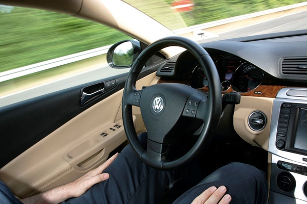
The responsibility always stays by driver even he is temporarily gets out of the control loop. He acts as an observer when TAP is active and can take back the vehicle control from TAP any time in safety-critical situations. The vehicle can also give back control to the driver if the preconditions for enabling TAP are not met. The driver is continuously monitored for drowsiness and attention by the vehicle to prevent accidents due to driving errors by an inattentive, distracted driver. The system also obeys overtaking rules and speed limits. Stop and start driving manoeuvres - for example in traffic jams - are also automated.
From time-to-market point of view a definitive advantage of the TAP system is that it has been realized on a relatively production-like sensors, consisting of production-level radar-, camera-, and ultrasonic-based sensors enhanced by a laser scanner and an electronic horizon. (Source: Volkswagen)
BMW demonstrated in 2009 that based on sensor fusion of eHorizon, GPS and samara information a vehicle can autonomously drive around a closed race circuit, following the ideal path. After the impressive performance BMW decided to introduce highly automated driving functions in series production vehicles until 2020. Aside typical functions like braking, accelerating and overtaking other vehicles entirely autonomously, the system will focus on challenges, like motorway intersections, toll stations, road works and national borders. The research prototype vehicle has run approximately 10,000 test kilometres up to now on public road with no driver intervention. (Source: [8])
Highly automated driving can also help in case of emergency, for example if biosensors detect that the driver is having a heart attack. The Emergency Stop Assistant function is able to switch the vehicle to highly automated driving mode and taking into account the traffic situation, manoeuvres the vehicle in a safe and controlled way to a standstill on the roadside. By switching on the hazard warning lights and making an eCall to request medical assistance, the situation is handled with maximum efficiently. (Source: [8])
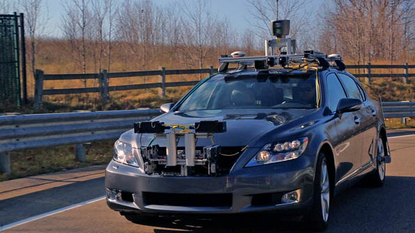
Toyota has presented its AHDA [9] test vehicle in 2013 that incorporates highly automated driving technologies to support safer highway driving and reduce driver workload. AHDA combines two automated driving technologies together Cooperative-adaptive Cruise Control and Lane Trace Control. The vehicle is fitted with cameras to detect traffic signals, radars and laser-scanner to detect vehicles, pedestrians, and obstacles in the surroundings. Via sensor fusion the vehicle is also able to identify traffic conditions, like intersections and merging traffic lanes.
In addition to radar based adaptive cruise control (ACC), Cooperative-adaptive Cruise Control (CCC) uses wireless communication between the vehicles to exchange vehicle dynamics data that enables smoother and more efficient control for maintaining a safe distance. Cooperative-adaptive Cruise Control uses 700-MHz band vehicle-to-vehicle ITS communications (V2V) to broadcast acceleration and deceleration data of the leading vehicle so that the following vehicles can control their speed profile correspondingly to better maintain inter-vehicle distance. Eliminating unnecessary accelerations and decelerations for the following vehicles results in better fuel efficiency and avoiding traffic congestion.
Lane Trace Control is a new assistance function that aids steering to keep the vehicle on an optimal driving path within the lane. It uses high-performance cameras, radar and sensor fusion to determine the optimal road path and provide smooth driving for the vehicle at all speeds. The system automatically intervenes in the steering, the drivetrain and the braking system when necessary to maintain the optimal path within the lane.
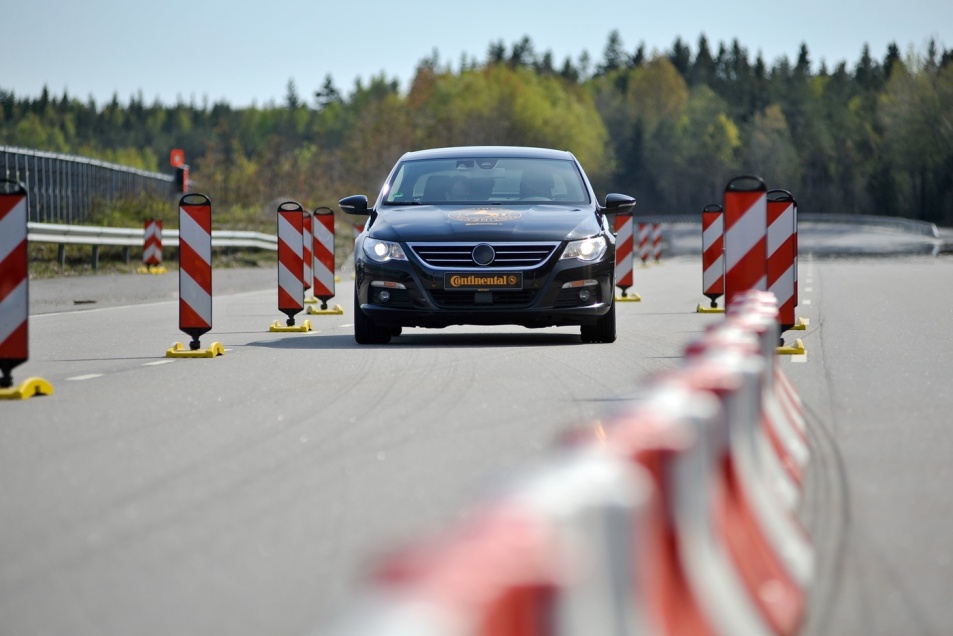
The objective of the automated assistance in road works and congestion function (developed within the EU funded HAVEit project) is to support the driver in overload situations like driving in narrow lanes of roadwork areas on motorways with lot of vehicles driving closely beside. Entering the road works and driving for longer distance in the road works area is very challenging for the driver. Some drivers even feel fear while other vehicles are driving so close in the parallel lane.
An integrated approach of the lateral and longitudinal control is used to adapt the speed and the lateral position of the vehicle to run the optimal path. (This assistance function will work at speeds between 0 and 80 km/h.) When the pre-conditions for the Automated Roadwork Assistance function are met the driver can switch to highly automated driving mode, taking his hands off the steering wheel. By this, the driver could drive through the road construction, without using his hands or feet. This guarantees that the driver gets the best possible support available, in particular with respect to lateral vehicle control.
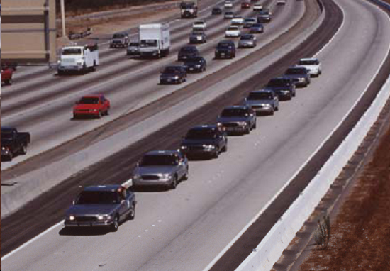
Another step in automation is the concept of platooning, which was motivated by intelligent highway systems and road infrastructure, see the PATH program in California and the MOC-ITS program in Japan. The European programmes were based on the existing road networks and infrastructure and focused mainly on commercial vehicles with their existing sensors and actuators. In a Hungarian project an automated vehicle platoon of heavy vehicles was developed. In a platoon system 5 to 10 vehicles are organized. The intervehicle spacing is small and constant at all speeds and vehicles. A well-organized platoon control may have advantages in terms of increasing highway capacity and decreasing fuel consumption and emissions. The control objective in platooning is to maintain vehicle following within the platoon and platoon stability under the constraint of comfortable ride. Since the desired intervehicle spacing is very small, the allowable position error is also small, which implies very accurate tracking of the desired spacing and speed trajectories. This accuracy puts constraints on the performance of the sensors and actuators as well as on the controller bandwidth.
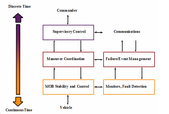
A three-layer software architecture that moves from discrete to continuous signals was in the PATH project, see Figure 20 and Figure 21. It should be noted that our design is not necessarily unique or optimal, but as a preliminary approach is sufficient to prove our point.
The stability and control layer deals with continuous signals and interfaces directly with the platform hardware. It contains several dynamic-positioning algorithms, a thruster allocation scheme, and sensor data processing and monitoring for fault detection. Control laws are given as vehicle state or observation feedback policies for controlling the vehicle dynamics. The corresponding events are sent to the manoeuvre coordination layer.
In the manoeuvre coordination layer control and observation subsystems responsible for safe execution of atomic manoeuvres such as assemble, split, wind tracking, and go to a location. Manoeuvres may include several modes according to the lattice of preferred operating modes. Mode changes are triggered by events generated by the stability layer monitors. It also monitors incidents and reacts to minimize their impact on manoeuvres and maximize safety.
The supervisory control layer: control strategies that the modules follow in order to minimize fuel consumption and maximize safety and efficiency. Discrete commands are given to achieve high-level goals of overall coordination and manoeuvring of the mobile offshore bases. This layer monitors the evolution of the system with respect to global mission goals. It receives commands and translates them into specific manoeuvres that the platforms need to carry out.
1.3.4. Full Automation
Until the driver has to be (legally) responsible for the behaviour of the vehicle, the driver will always be an integral part of the control loop. That is why full automation of public road vehicles is not realistic in the near future. There are some promising experiments on fully automated manoeuvring of vehicles but most of them are realized on a separated area and are far from being able to adapt on public roads without an intelligent, independent road infrastructure.
Distinguished members of IEEE, the world’s largest professional organization dedicated to advancing technology for humanity, have selected autonomous vehicles as the most promising form of intelligent transportation, anticipating that they will account for up to 75 % of cars on the road by the year 2040, see [10].
The U.S. government also supports the autonomous car research, as keeping it the next evolutionary step in technology. In Nevada, Florida and California it is licensed to test vehicles without a driver, which is used by Google as getting the first self-driven car license in Nevada in 2012. (Source: [11])
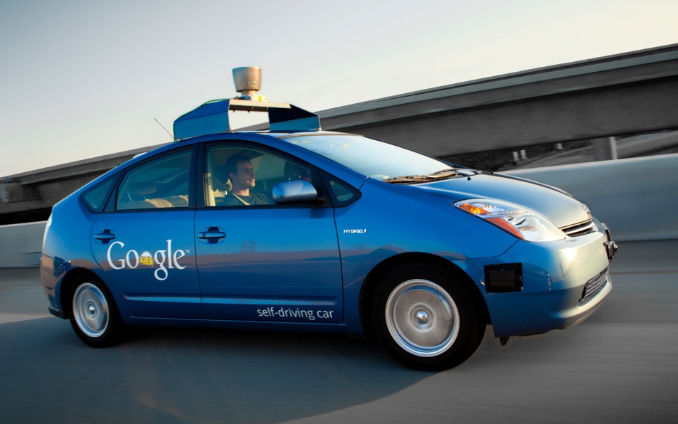
Google gathered the best engineers from the DARPA Challenge series, which was a legendary competition for American autonomous vehicles. It was started in 2004, funded by the Defense Advanced Research Projects Agency, which is a research institute of United States Department of Defense. Three events were held in 2004, 2005 and 2007 regarding to the autonomous passenger cars. The 2012 event has focused on autonomous emergency-maintenance robots.
Google’s self-driving car use video cameras, radar sensors and a LIDAR (see Section 3) for environment sensing, as well as detailed maps for navigation. The car is supported by the Google’s data centres, which can process the information gathered by the test cars when mapping the terrain. (Source: [12])
The main vehicle manufacturers are also heading toward the autonomous solutions, but they are trying to reach the goal step-by-step, and not at once like Google. They are developing (in cooperation with their OEMs) such subsystems which can increase the automation level of the car, and also can be marketed in production vehicles as new driver assistance systems. An example of this attitude can be found in an interview with Daimler head of development Thomas Weber, who said "Autonomous driving will not come overnight, but will be realized in stages". The plans to start selling self-driving cars is about 2020, primarily in North America. (Source: [13])
Chapter 2. Layers of integrated vehicle control
Conventionally, the control systems of vehicle functions to be controlled are designed separately by the equipment manufacturers and component suppliers. One of the problems of independent design is that the performance demands, which are met by independent controllers, are often in interaction or even conflict with each other in terms of the full vehicle. As an example braking during a vehicle manoeuvre modifies the yaw and lateral dynamics, which requires parallel steering action or, as another example, under/over steering requires parallel braking intervention. The second problem is that both hardware and software will become more complex due to the dramatically increased number of sensors and signal cables and these solutions can lead to unnecessary hardware redundancy.
The demand for the integrated vehicle control methodologies including the driver, vehicle and road arises at several research centres and automotive suppliers. The principle of integrated control with the CAN network was presented by Kiencke in [14]. The purpose of integrated vehicle control is to combine and supervise all controllable subsystems affecting vehicle dynamic responses. An integrated control system is designed in such a way that the effects of a control system on other vehicle functions are taken into consideration in the design process by selecting the various performance specifications. Recently, several important papers have been presented in this topic, see e.g. [15][16][17][18][19].
2.1. Levels of intelligent vehicle control
The complex tasks of a vehicle control must be structured in a way that the logical steps are built on one another and the complexity can be simplified by abstracting substructures. The levels of intelligent vehicle control defined by Prof. Palkovics [20] is suitable to provide a general overview of the subject, later the different layers of intelligent vehicle control are described in a way they depend on each-other.
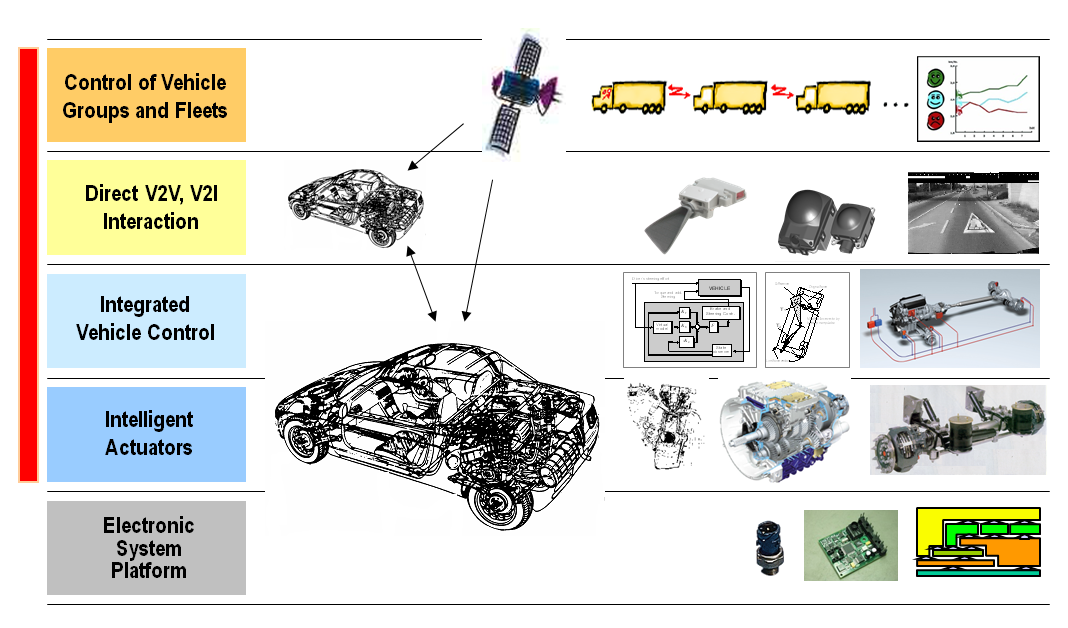
2.1.1. Electronic System Platform
The bottom level, the “Electronic System Platform“ solutions contain all the necessary building elements that are required for building up an electronically controlled vehicle system. This includes basic electronic and mechatronic hardware components like sensors and actuators, includes ECUs, but also software components like operating systems, diagnostics software, peripheral drivers and so on. The platform characteristics lies behind the fact that these individual components, building block can be used widespread in different makes and vehicle types, resulting in high production volume, thus reliable design and low costs.
2.1.2. Intelligent Actuators
The second level, the “Intelligent Actuators“ are the electronically controllable separate five main units of the vehicle drivetrain, namely the engine, transmission, suspension, brake system and the steering system. These main units are individual intelligences meaning that each unit has its own ECU with sophisticated functionality for electronic control in itself having communication links (CAN, FlexRay) to other ECUs for interaction, but one ECU is only responsible for the control of one unit. Typical characteristics of the intelligent actuators are having a dedicated interface for the electronic control of the whole unit. This is why they are often called as „by-wire“ systems, meaning that there is no mechanical connection for the control. In this case these units are referred as drive-by-wire, shift-by-wire, suspension-by-wire, brake-by-wire abs last but not least steer-by-wire systems in a vehicle. These actuators are “must have” components for the intelligent vehicle control.
2.1.3. Integrated Vehicle Control
In the next level, in the “Integrated Vehicle Control” there is a harmonized control of the intelligent actuators (instead of individual control) on a vehicle level. This layer has an influence on the whole vehicle motion. Maybe it is not trivial, but it is easy to understand what synergies become available in cases of harmonized or in other words integrated control of the intelligent actuators. The most obvious example is the integrated control of the brake and steering system, where the harmonized control could result in a significantly shorter brake distance. Let us imagine a so called u-split situation, where the road surface is divided into two parts based on a longitudinal separation. In this case the vehicles left hand side wheels (front left, rear left) are running on a hi-u surface e.g. u=0,8, while the right hand side wheels (front right, rear right) are running on a low-u surface e.g. u=0,1. In this case there is a great potential for synergy when the brake system realizes the u-split situation and instead of using “select-low” strategy – meaning that the lower u surface determines the maximum brake force on each sides – uses the maximum allowable braking force on each side with the help of the steering system providing compensating yaw torque to stabilize the vehicle direction.
2.1.4. Direct V2V, V2I Interactions
The fourth levels called “Direct V2V, V2I Interactions” where ad-hoc direct vehicle-to-vehicle (V2V) communications and ad-hoc direct vehicle-to-infrastructure (V2I) communications support the vehicle and its driver to be able to carry out the control task, safely and economically. The control is based on the relative position of the other vehicles or the elements of the infrastructure. The simplest example of these interactions is the Adaptive Cruise Control (ACC) function, where the distance and the velocity of the following vehicle is determined by a radar system, establishing ad-hoc direct V2V connection between the ego and the following vehicle. The ACC function is (currently) limited to the longitudinal direction, but such communication interactions can be established also in the lateral direction for e.g. automated trajectory planning. A currently market available example for ad-hoc direct V2I interaction is the automatic traffic sign recognition function.
2.1.5. Control of Vehicle Groups and Fleets
Last but not least there is the fifth level with “Control of Vehicle Groups and Fleets”. This layer covers the control of a whole vehicle flow or a partial set of the vehicles, where the grouping is based on either the current location or on the vehicle ownership (fleets).Good example for the location based selection of the vehicle groups is the control of a road cross section or the so called platooning, where an ad-hoc virtual road train is formulated on a highway. Transportation fleets are generally controlled via a centralized informatics system, where current market availability is rather logistics, delivery control and vehicle operation related information acquisition (FMS, Telematics) than remote movement control of the vehicles.
The above described structuring of the intelligent vehicle control is rather system oriented while the following part will mostly concentrate on the internal control structure of a vehicle.
2.2. Layers of vehicle control
For achieving an integrated control a possible solution could be to set the design problem for the whole vehicle and include all the performance demands in a single specification. Besides the complexity of the resulting problem, which cannot be handled by the existing design tools, the formulation of a suitable performance specification is the main obstacle for this direct global approach. In the framework of available design techniques formulation and successful solution of complex multi-objective control tasks are highly nontrivial.
From control design point-of-view the integrated vehicle control consists of five potentially distinct layers[16]:
The physical layout of local control based on hardware components, e.g. ABS/EBS, TCS, TRC, suspension.
Layout of simple control actions, e.g. yaw/roll stability, ride comfort, forward speed.
The connection layout of information flow from sensors, state estimators, performance outputs, condition monitoring and diagnostics.
The layout of control algorithms and methodologies with fault-tolerant synthesis, e.g. lane detection and tracking, avoiding obstacles
Layout of the integrated control design.
Research into integrated control basically focuses on the fifth layers; however the components of any integration belong to the third and fourth layer. The components in the first two layers are assumed to exist. Note, that to some extent the layers may be classified by the degree of centralization, e.g. centralized, supervisory or decentralized.
During the implementation of the designed control algorithms additional elements from information technology and communication will be included in the control process. In the classical control algorithms a lossless link is assumed to exist between the system and control these algorithms are concerned mostly with delays, parametrical uncertainties, measurement noise and disturbances.
The performance of the implemented control is heavily affected by the presence of the communication mechanism (third layer), the network sensors and actuators, distributed computational algorithms or hybrid controllers. It is useful to incorporate knowledge about the implementation environment during the controller design process, for example dynamic task management, adaptability to the state (faults) of sensors and actuators, the demands imposed by a fault tolerant control, the structural changes occurring in the controlled system.
From architectural design point of view the model based simulation of the planned architecture provides an early stage feedback about the potential bottlenecks in the design [21] [22]. Early stage simulation can reveal hidden mistakes that could turn out only after system implementation. When modification should be made on the implemented system due to the results of the safety analysis, it has much higher costs. The simulation based analysis needs lower costs, but takes time to prepare and carry out the simulations. The main advantage is that the simulation based analysis can be carried out from the early stage of the development. Certainly at the beginning of a system development, the system architecture is in its initial stage; therefore simulation model may also be inaccurate. The system design engineering and the safety engineering are parallel processes; the system model for the safety simulations is getting more and more accurate during the development. And there is a continuous feedback from the safety engineering to the system design engineering [23][24].
The software technology is not simply a software implementation of the control algorithm. The implementation and the software/hardware environment are also a dynamic system, which has an internal state and which respond to inputs and produces outputs. If the actual plant is combined with an embedded controller through the sensor and actuator dynamics, a distributed hybrid system is created. With this approach the control design is closely connected with software design. The control design is evolving through the development of hybrid optimal control, observability/controllability analysis, and software design is being facilitated by distributed computing and messaging services, real-time operating systems and distributed object models.
In the different prototype implementation of autonomous or highly automated vehicles a strictly defined layer structure can be observed that definitely corresponds to the above mentioned layer structure even if some layers are merged together for simplicity. The following figure shows the PEIT approach of the vehicle control layer structure[25]:
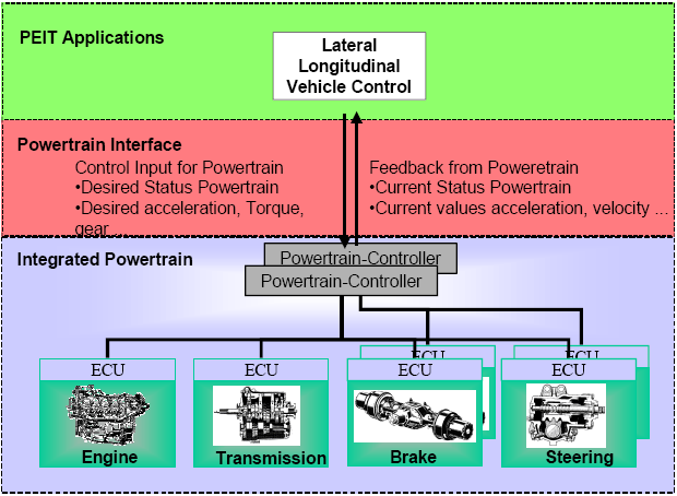
The PEIT architecture differentiates 3 different layers, namely the PEIT application layer, the powertrain interface and the integrated powertrain layer. The integrated powertrain layer contains 4 intelligent actuators, the drive-by-wire, the shift-by-wire, the brake-by-wire and the steer-by-wire systems. Important to notice that in the PEIT architecture the engine and transmission actuators are single subsystems, while the brake and steering systems are redundant subsystems. This is due to the requirement of availability based on the safety critical categorization of the subsystems. In case of the engine there is no backup function, in case of a transmission system there is only a “limp home” function which serves as a limited (e.g. one fixed gear) but useful functionality to maintain the movability of the vehicle. When it comes to the brake or the steering system it is obvious that any malfunction can result in serious consequences, so these systems must be designed in a way that they tolerate at least one failure. This is why safety critical systems have fault-tolerant architecture. There are different possible realizations of a fault tolerant system, one is simply using redundancy. In this case there are two parallel system elements that work simultaneously and in case of a failure one system can take over the control from the broken one. There is also a redundant powertrain controller can be found in the integrated powertrain layer, further dividing the layer into 2 sublayers. Referring back to the Prof. Palkovics the powertrain controller implements the vehicle level control, while the by-wire systems underneath are the intelligent actuators.
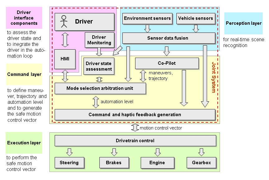
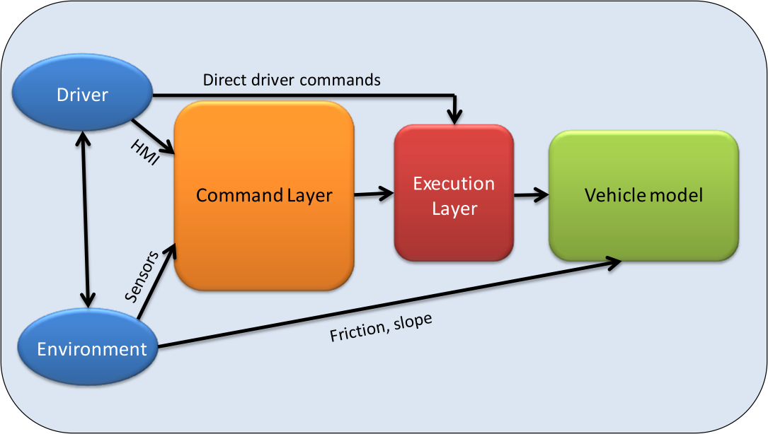
The HAVEit layer structure [6] is a further optimized, extended and structured architecture, where there are basically two main layers, namely the command layer and the execution layer. The interface in between is specifically called the “motion vector”. Even if there are a lot of other functions involved, the basic idea is that the command layer specifies the motion vector, which has to be followed by the vehicle that is carried out by the execution layer.
2.2.1. Command layer
The command layer contains the high level algorithms for the longitudinal and the lateral control of the automated vehicle. The command layer calculates the desired acceleration and direction and communicates the results to the powertrain via the powertrain interface, which also provides feedback about the vehicle state for the high level control.
Based on the driver intention and the information coming from the perception layer the command layer defines the vehicle automation level and calculates the vehicle trajectory. The objective of the perception layer is to collect information about the external environment and the vehicle, thus providing information about vehicle status and objects in the surrounding environment. From this information the command layer determines the obtainable levels of vehicle automation and displays the options to the driver. Meanwhile the co-pilot calculates possible vehicle trajectories and prioritizes them based on the accident risk. The driver selects the desired level of vehicle automation from the available options via the HMI. Finally the mode selection unit decides the level of automation and selects the trajectory to be executed.
2.2.2. Motion Vector
The motion vector acts as an interface between the command layer and the execution layer. It is bidirectional, delivering longitudinal and lateral control commands to the powertrain and providing vehicle status feedback information for the higher level control.
This middle layer contains predefined data transfer for the control and the feedback of the powertrain. It includes commands for the vehicle control including the desired status of the powertrain and the required acceleration and torque. This interface also includes status feedback from the powertrain to the application layer providing important information whether the control action resulted in the required movement.
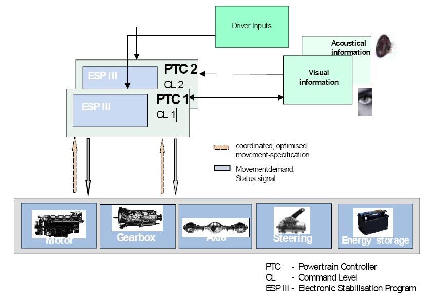
2.2.3. Execution Layer
The execution layer contains a full drivetrain control connected to intelligent actuators via a high speed communication network. As the implementation of a fully electronic interface (motion vector) for controlling the powertrain enables the replacement of the human driver for an electronic intelligence (auto-pilot), the execution layer cannot distinguish whether the commands are originated from a human driver or an auto-pilot. The commands are coming through the same interface, so the execution layer has to execute only. Considering that there are safety critical subsystems can be found among the intelligent actuators a fault-tolerant architecture is a prerequisite. This fault tolerant architecture not only includes duplicated powertrain controllers, steering and braking systems but also a redundant communication network, power supply and HMI to the driver. The following figure shows the powertrain control structure of the execution layer in the PEIT demonstrator vehicle[25].
2.3. Integrated control
Conventionally, the control systems of vehicle functions to be controlled are designed separately by the equipment manufacturers and component suppliers. One of the problems of independent design is that the performance demands, which are met by independent controllers, are often in interaction or even conflict with each other in terms of the full vehicle. As an example braking during a vehicle manoeuvre modifies the yaw and lateral dynamics, which requires steering action or, as another example, under/oversteering requires braking intervention. The second problem is that both hardware and software will become more complex due to the dramatically increased number of sensors and signal cables and these solutions can lead to unnecessary hardware redundancy.
The demand for the integrated vehicle control methodologies including the driver, vehicle and road arises at several research centres and automotive suppliers. The principle of integrated control with the CAN network was presented by Kiencke in [3]. The purpose of integrated vehicle control is to combine and supervise all controllable subsystems affecting vehicle dynamic responses. An integrated control system is designed in such a way that the effects of a control system on other vehicle functions are taken into consideration in the design process by selecting the various performance specifications. Recently, several important papers have been presented in this topic, see e.g. [4], [5], [6], [7], [8].
For achieving an integrated control a possible solution could be to set the design problem for the whole vehicle and include all the performance demands in a single specification. Besides the complexity of the resulting problem, which cannot be handled by the existing design tools, the formulation of a suitable performance specification is the main obstacle for this direct global approach. In the framework of available design techniques formulation and successful solution of complex multi-objective control tasks are highly nontrivial. Another solution to the integrated control is a decentralized control structure, in which there is a logical relationship between the individually-designed controllers. The communication between control components is performed by using the CAN bus (see Section 7.1). The advantage of this solution is that the components with their sensors and actuators can be designed by the suppliers independently. However, the local controllers require a group of sensors and hardware components, which may lead to different redundancies. The difficulty in the decentralized structure is that the control design leads to hybrid and switching methods with a large number of theoretical problems, see [8],[9],[10],11]. While stability of the control scheme assuming arbitrary switching can be ensured by imposing suitable dwell-times, it is hard to guarantee a prescribed performance level in general in the design process.
In more detail it means that
multiple-objective performance from available actuators must be improved,
sensors must be used in several control tasks,
the number of independent control systems must be reduced, at the same time the flexibility of the control systems must be improved by using plug-and-play extensibility.
These principles are close to the low-cost demands of the vehicle industry. In this way it should be possible to generate redundancy in a distributed way at the system level, which is cheaper and more effective than simply duplicating key components.
The integrated control consists of five potentially distinct levels:
The physical layout of local control based on hardware components, e.g. ABS/EBS, TCS, TRC, suspension.
Layout of simple control actions, e.g. yaw/roll stability, ride comfort, forward speed.
The connection layout of information flow from sensors, state estimators, performance outputs, condition monitoring and diagnostics.
The layout of control algorithms and methodologies with fault-tolerant synthesis, e.g. lane detection and tracking, avoiding obstacles
Layout of the integrated control design.
Research into integrated control basically focuses on the fifth layer, however the components of any integration belong to the third and fourth layers. The components in the first two layers are assumed to exist. Note, that to some extent the layers may be classified by the degree of centralization, e.g. centralized, supervisory or decentralized.
During the implementation of the designed control algorithms additional elements from information technology and communication will be included in the control process. In the classical control algorithms a lossless link is assumed to exist between the system and control these algorithms are concerned mostly with delays, parametrical uncertainties, measurement noise and disturbances.
The performance of the implemented control is heavily affected by the presence of the communication mechanism, the network sensors and actuators, distributed computational algorithms or hybrid controllers. It is useful to incorporate knowledge about the implementation environment during the controller design process, for example dynamic task management, adaptability to the state (faults) of sensors and actuators, the demands imposed by a fault tolerant control, the structural changes occurring in the controlled system.
The software technology is not simply a software implementation of the control algorithm. The implementation and the software/hardware environment are also a dynamic system, which has an internal state and which respond to inputs and produces outputs. If the actual plant is combined with an embedded controller through the sensor and actuator dynamics, a distributed hybrid system is created. With this approach the control design is closely connected with software design. The control design is evolving through the development of hybrid optimal control, observability/controllability analysis, and software design is being facilitated by distributed computing and messaging services, real-time operating systems and distributed object models.
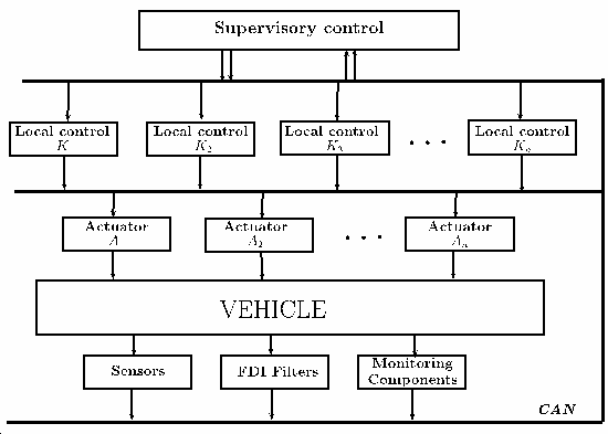
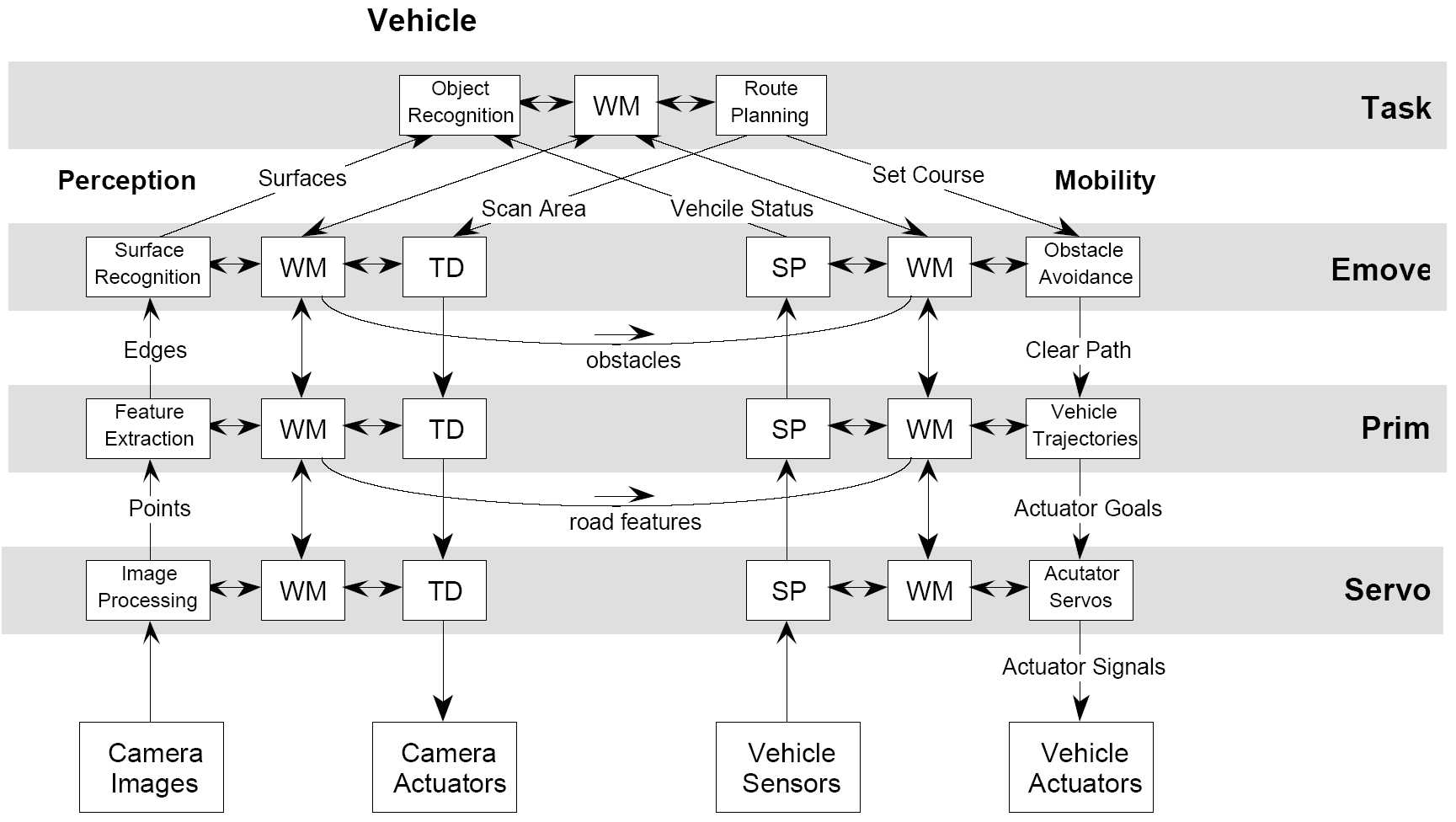
A reference control architecture for autonomous vehicles is presented in Figure 27. It shows how the software components should be identified and organized. This reference model is based on the general Real-time Control System (RCS) Reference Model Architecture, and has been applied to many kinds of applications, including autonomous vehicle control.
2.4. Distributed control structure
Another solution to the integrated control is a distributed (decentralized) control structure, in which there is a logical relationship between the individually-designed controllers. The communication between control components is performed by using the vehicle communication network (e.g. CAN bus). The advantage of this solution is that the components with their sensors and actuators can be designed by the suppliers independently. However, the local controllers require a group of sensors and hardware components, which may lead to different redundancies. The difficulty in the distributed structure is that the control design leads to hybrid and switching methods with a large number of theoretical problems, see [19][26][27][28]. While stability of the control scheme assuming arbitrary switching can be ensured by imposing suitable dwell-times, it is hard to guarantee a prescribed performance level in general in the design process.
Integrated control based on a distributed (decentralized) structure means that
multiple-objective performance from available actuators must be improved,
sensors must be used in several control tasks,
the number of independent control systems must be reduced, at the same time the flexibility of the control systems must be improved by using plug-and-play extensibility
These principles are close to the low-cost demands of the vehicle industry. In this way it should be possible to generate redundancy in a distributed way at the system level, which is cheaper and more effective than simply duplicating key components.
Chapter 3. Environment Sensing (Perception) Layer
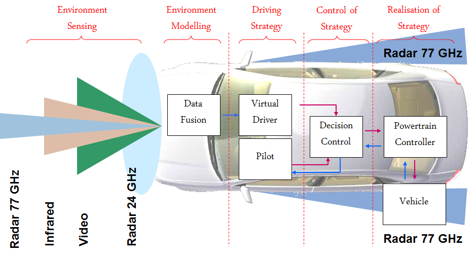
The task of the environment sensing layer is to provide comprehensive information about the surrounding objects around the vehicle. There are different types of sensors installed all around the vehicle that deliver information from near, medium and distant ranges. The following figure shows the elements of the environment sensing around the vehicle.
The vehicle sensor devices can be classified according to the aforementioned viewpoints:
Near distance range
Radar (24GHz)
Video
3D Camera
Medium distance range
Video
Far distance range
Radar (77/79GHz)
Lidar
3.1. Radar
Automotive radar sensors are responsible for the detection of objects around the vehicle and the detection of hazardous situations (potential collisions). A positive detection can be used to warn/alert the driver or in higher level of vehicle automation to intervene with the braking and other controls of the vehicle in order to prevent an accident. The basic theory of radar systems is explained in the following chapters based on [29].
In an automotive radar system, one or more radar sensors detect obstacles around the vehicle and their speeds relative to the vehicle. Based on the detection signals generated by the sensors, a processing unit determines the appropriate action needed to avoid the collision or to reduce the damage (collision mitigation).
Originally the word radar is an acronym for RAdio Detection And Ranging. The measurement method is the active scanning i.e. the radar transmits radio signal and the reflected signal is analysed. The main advantages of the radar are the lower costs and the weather-independency.
The basic output information of the automotive radars is the followings:
Detection of objects
Relative position of the objects to the vehicle
Relative speed of the objects to the vehicle
Based on this information the following user-level functionalities can be implemented:
Alert the driver about any potential danger
Prevent collision by intervening with the control of the vehicle in hazardous situations
Take over partial control of the vehicle (e.g., adaptive cruise control)
Assist the driver in parking the car
Radar operation can be divided into two major tasks:
Distance detection
Relative speed detection
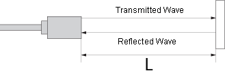
Distance detection can be performed by measuring the round-trip duration of a radio signal. Based on the wave speed in the medium, it will take a certain time for the transmitted signal to travel, be reflected from the target, and travel back to the radar receiver. By measuring this time interval that the signal has travelled the distance can easily be calculated.
The underlying concept in the theory of speed detection is the Doppler frequency shift. A reflected wave from a moving object will experience a frequency change, depending on the relative speed and direction of movement of the source that has transmitted the wave and the object that has reflected the wave. If the difference between the transmitted signal frequency and received signal frequency can be measured, the relative speed can also be calculated.
According to the type of transmission the radar system can be continuous wave (CW) or pulsed. In continuous-wave (CW) radars, a high-frequency signal is transmitted and by measuring the frequency difference between the transmitted and the received signal (Doppler frequency), the speed of the reflector object can be quite well estimated.
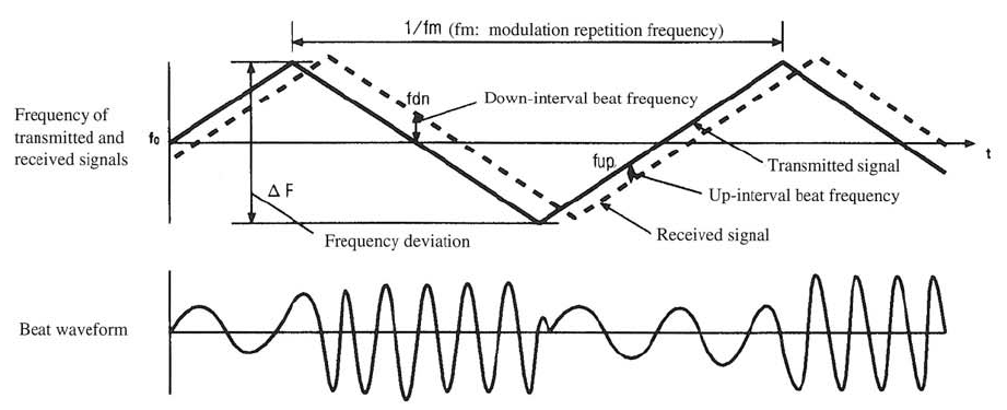
The most widely used technology is the FM-CW (Frequency Modulated Continuous Wave). In FMCW radars, a ramp waveform or a saw-tooth waveform is used to generate a signal with linearly varying frequency in time domain. The high-frequency transmitted signal emitted from the sensor is modulated using a frequency f0, modulation repetition frequency is fm, and frequency deviation is ΔF. The radar signal is reflected by the target, and the radar sensor receives the reflected signal. Beat signals (see Figure 32 [30]) are obtained from the transmitted and received signals and the beat frequency is proportional to the distance between the target and the radar sensor. Relative speed and relative distance can be determined by measuring the beat frequencies.
In pulsed radar architectures, a number of pulses are transmitted and from the time delay and change of pulse width that the transmitted pulses will experience in the round trip, the distance and the relative speed of the target object can be estimated. Transmitting a narrow pulse in the time domain means that a large amount of power must be transmitted in a short period of time. In order to avoid this issue, spread spectrum techniques may be used.
There are 4 major frequency bands allocated for radar applications, which can be divided into two sub-categories: 24-GHz band and 77-GHz band.
The 24-GHz band consists of two sub-bands, one around 24.125GHz with a bandwidth of around 200MHz and, the other around 24GHz with a bandwidth of 5GHz. Both of these bands can be used for short/mid-range radars.
The 77-GHz band also consists of two sub-bands, 76-77GHz for narrow-band long-range radar and 77-81GHz for short-range wideband radar (see Figure 33 [29]).
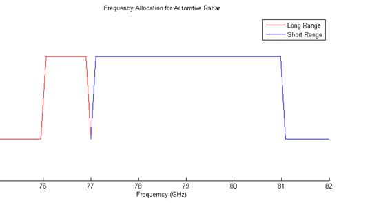
As frequency increases, smaller antenna size can be utilized. As a result, by going toward higher frequencies angular resolution can be enhanced. Furthermore, by increasing the carrier frequency the Doppler frequency also increases proportional to the velocity of the target; hence by using mm-wave frequencies, a higher speed resolution can be achieved. Range resolution depends on the modulated signal bandwidth, thus wideband radars can achieve a higher range resolution, which is required in short-range radar applications. Recently, legal authorities are pushing for migration to mm-wave range by imposing restrictions on manufacturing and power emission in the 24GHz band. It is expected that 24-GHz radar systems will be phased out in the next few years (at least in the EU countries). This move will help eliminate the issue of the lack of a worldwide frequency allocation for automotive radars, and enable the technology to become available in large volumes.
By using the 77-GHz band for long-range and short-range applications, the same semiconductor technology solutions may be used in the implementation of both of them. Also, higher output power is allowed in this band, as compared to the 24-GHz radar band. 76-77-GHz and 77-81-GHz radar sensors together are capable of satisfying the requirements of automotive radar systems including short-range and long-range object detection. For short-range radar applications, the resolution should be high; as a result, a wide bandwidth is required. Therefore, the 77-81-GHz band is allocated for short-range radar (30-50m). For long-range adaptive cruise control, a lower resolution is sufficient; as a result, a narrower bandwidth can be used. The 76-77-GHz is allocated for this application.
As an explanation of the above mentioned range classification, the automotive radar systems can be divided into three sub-categories: short-range, mid-range and long-range automotive radars. For short-range radars, the main aspect is the range accuracy, while for mid-range and long-range radar systems the key performance parameter is the detection range.
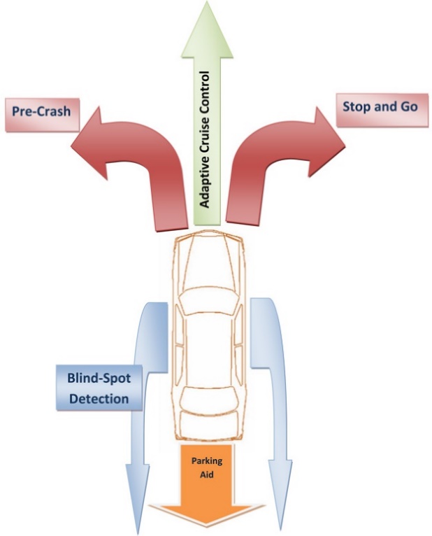
Short-range and mid-range radar systems (range of tens of meters) enable several applications such as blind-spot detection and pre-crash alerts. It can also be used for implementation of “stop–and-go” traffic jam assistant applications in city traffic.
Long-range radars (hundreds of meter) are utilized in adaptive cruise-control systems. These systems can provide enough accuracy and resolution for even relatively high speeds.
Nowadays the most significant OEMs can integrate the radar functionality into a small and relatively low cost device. When Bosch upgraded Infineon's product during the development of its third-generation long-range radar (dubbed, unimaginatively, the LRR3), both the minimum and maximum ranges of its system got better: The minimum range dropped from 2 meters to half a meter, and the maximum range shot from 150 to 250 meters. At the same time, the detection angle doubled to 30 degrees, and the accuracy of angle and distance measurements increased fourfold. The superiority originates from the significantly higher radar bandwidth used in the systems containing the silicon-based chips. Another point is the new system's compact size—just 7.4 by 7 by 5.8 centimetres.
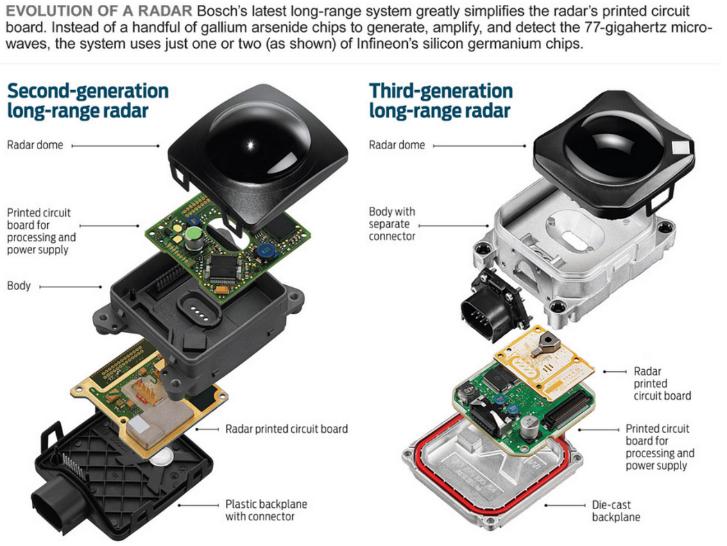
The system utilizes four antennas and a big plastic lens to shoot microwaves forward and also detect the echoes, meanwhile ramping the emission frequency back and forth over 500-MHz band. (Because the ramping is so fast, the chance of two or more radars interfering is extraordinarily low.) The system compares the amplitudes and phases of the echoes, pinpointing each car within range to within 10 cm in distance and 0.1 degree in displacement from the axis of motion. Then it works out which cars are getting closer or farther away by using the Doppler Effect. In all, the radar can track 33 objects at a time. (Source[31])
The following table shows the main properties of the Continental’s ARS300 Long- and Mid-range Rader.
Range (Measured using corner reflector, 10 m² RCS) | 0.25m up to 200m far range scan 0.25m up to 60m medium range scan |
Field of view | field of view conform with the ISO classes I ... IV azimuth 18° far range scan 56° medium range scan elevation 4.3° (6dB beam width) |
Cycle time | 66 ms (far and medium range scan in one cycle) |
Accuracy | range 0.25m, no ambiguities angle 0.1° complete far distance field of view 1.0° medium range (0° < || < 15°) 2.0° medium range (15° < || < 25°) speed (-88 km/h ... +265 km/h; extended to all realistic velocities by tracking software) 0.5 km/h |
Resolution | range 0.25m (d < 50m) 0.5m (50m < d < 100m) 1m (100m < d < 200m) |
3.2. Ultrasonic
Ultrasonic sensors are industrial control devices that use sound waves above 20 000 Hz, beyond the range of human hearing, to measure and calculate distance from the sensor to a specified target object. This sensor technology is detailed here from [32].
The sensor has a ceramic transducer that vibrates when electrical energy is applied to it. This phenomenon is called piezoelectric effect. The word piezo is Greek for "push". The effect known as piezoelectricity was discovered by brothers Pierre and Jacques Curie when they were 21 and 24 years old in 1880. Crystals which acquire a charge when compressed, twisted or distorted are said to be piezoelectric. This provides a convenient transducer effect between electrical and mechanical oscillations. Quartz demonstrates this property and is extremely stable. Quartz crystals are used for watch crystals and for precise frequency reference crystals for radio transmitters. Rochelle salt produces (Potassium sodium tartrate) a comparatively large voltage upon compression and was used in early crystal microphones. Several ceramic materials are available which exhibit piezoelectricity and are used in ultrasonic transducers as well as microphones. If an electrical oscillation is applied to such ceramic wafers, they will respond with mechanical vibrations which provide the ultrasonic sound source.
The vibrations compress and expand air molecules in waves from the sensor face to a target object. A transducer both transmits and receives sound. The ultrasonic sensor will measure distance by emitting a sound wave and then listening for a set period of time, allowing for the return echo of the sound wave bouncing off the target before retransmitting (pulse-echo operation mode).
The sensor emits a packet of sonic pulses and converts the echo pulse into a voltage. The controller computes the distance from echo time and the velocity of sound. The velocity of sound in the atmosphere reaches 331.45 m/s when the temperature is 0°C. The sound velocity at different temperatures can be calculated with the following formula. Sound velocity increases by 0.607 m/s every time the temperature rises 1°C.
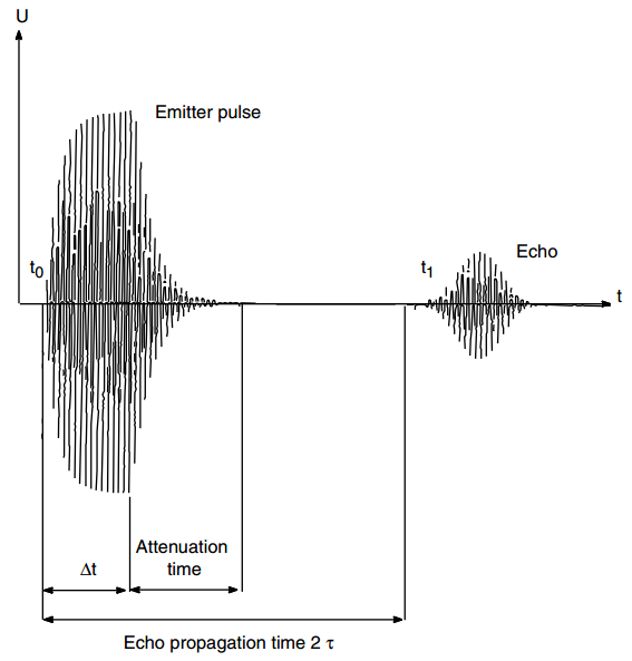
The emitted pulse duration Δt and the attenuation time of the sensor result in an unusable area in which the ultrasonic sensor cannot detect and object. That is why the limited minimum detection range is around 20 cm.
Ultrasonic sensors use sound rather than light for detection, they work in applications where photoelectric sensors may not. Ultrasonic sensors are a great solution for clear object detection and for liquid level measurement, applications that photoelectric struggle with because of target translucence. Target colour and/or reflectivity don't affect ultrasonic sensors which can operate reliably in high-glare environments. Ultrasonic sensors definitely have advantages when sensing clear objects, liquid level or highly reflective or metallic surfaces. Ultrasonic sensors also function well in wet environments where as an optical beam may refract off the water droplets. On the other hand ultrasonic sensors are susceptible to temperature fluctuations or wind.
In the automotive industry the ultrasonic sensors are mainly used for parking aid and blind-spot functions. These sensors typically work at ~48 kHz operating frequency with a detection range of 25-400 cm. The opening angle is about 120° horizontally and 60° vertically.
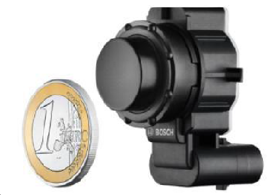
The general architecture of automotive ultrasonic systems is shown on Figure 38. It consists of the ultrasonic sensors mounted into the front and rear bumpers, the analogue amplifiers and filters and the ECU. The main unit of the ECU (generally a microcontroller) generates the signal and drives the sensors by the power amplifier. The generated sound wave reflects off an object and is converted back to electronic signal with the same sensor element. The MCU measures the echo signal, evaluates and calculates the distances. Generally the results are broadcasted by high-level communication interface such as CAN, or sent directly to an HMI for further processing.
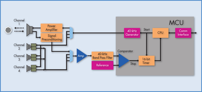
3.3. Video camera
The recording capabilities of the automotive video cameras are based on image sensors (imagers). It is the common name of those digital sensors which can convert an optical image into electronic signals. Currently used imager types are semiconductor based charge-coupled devices (CCD) or active pixel sensors formed of complementary metal–oxide–semiconductor (CMOS) devices. These main image capture technologies are introduced based on the comparison in [33].
Both image sensors are pixelated semiconductor structures. They accumulate signal charge in each pixel proportional to the local illumination intensity, serving a spatial sampling function. When exposure is complete, a CCD (Figure 39 [33]) transfers each pixel’s charge packet sequentially to a common output structure, which converts the charge to a voltage, buffers it and sends it off-chip. In a CMOS imager (Figure 40 [33]), the charge-to-voltage conversion takes place in each pixel. This difference in readout techniques has significant implications for sensor architecture, capabilities and limitations.
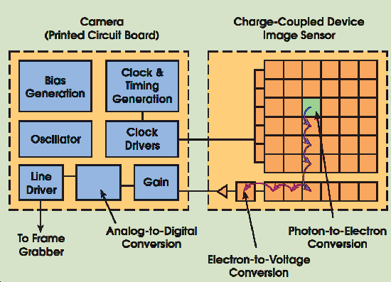
On a CCD, most functions take place on the camera’s printed circuit board. If the application demands hardware modifications, a designer can simply change the electronics without redesigning the imager.
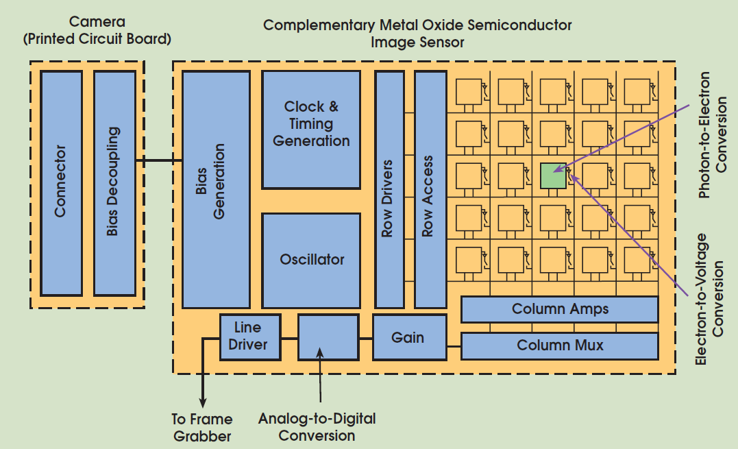
A CMOS imager converts charge to voltage at the pixel, and most functions are integrated into the chip itself. This makes imager functions less flexible but, for applications in rugged environments, a CMOS camera can be more reliable.
3.3.1. Image sensor attributes
As defined in [33] there are eight attributes that characterize image sensor performance. This attributes will be explained in details in the following paragraphs:
Responsivity, the amount of signal the sensor delivers per unit of input optical energy. CMOS imagers are marginally superior to CCDs, in general, because gain elements are easier to place on a CMOS image sensor. Their complementary transistors allow low-power high-gain amplifiers, whereas CCD amplification usually comes at a significant power penalty. Some CCD manufacturers are challenging this concept with new readout amplifier techniques.
Dynamic range, the ratio of a pixel’s saturation level to its signal threshold. It gives CCDs an advantage by about a factor of two in comparable circumstances. CCDs still enjoy significant noise advantages over CMOS imagers because of quieter sensor substrates (less on-chip circuitry), inherent tolerance to bus capacitance variations and common output amplifiers with transistor geometries that can be easily adapted for minimal noise. Externally coddling the image sensor through cooling, better optics, more resolution or adapted off-chip electronics cannot make CMOS sensors equivalent to CCDs in this regard.
Uniformity, the consistency of response for different pixels under identical illumination conditions. Ideally, behaviour would be uniform, but spatial wafer processing variations, particulate defects and amplifier variations create non-uniformities. It is important to make a distinction between uniformity under illumination and uniformity at or near dark. CMOS imagers were traditionally much worse under both regimes. Each pixel had an open-loop output amplifier, and the offset and gain of each amplifier varied considerably because of wafer processing variations, making both dark and illuminated non-uniformities worse than those in CCDs. Some people predicted that this would defeat CMOS imagers as device geometries shrank and variances increased. However, feedback-based amplifier structures can trade off gain for greater uniformity under illumination. The amplifiers have made the illuminated uniformity of some CMOS imagers closer to that of CCDs, sustainable as geometries shrink. Still lacking, though, is offset variation of CMOS amplifiers, which manifests itself as non-uniformity in darkness. While CMOS imager manufacturers have invested considerable effort in suppressing dark non-uniformity, it is still generally worse than that of CCDs. This is a significant issue in high-speed applications, where limited signal levels mean that dark non-uniformities contribute significantly to overall image degradation.
Shuttering, the ability to start and stop exposure arbitrarily. It is a standard feature of virtually all consumer and most industrial CCDs, especially interline transfer devices, and is particularly important in machine vision applications. CCDs can deliver superior electronic shuttering, with little fill-factor compromise, even in small-pixel image sensors. Implementing uniform electronic shuttering in CMOS imagers requires a number of transistors in each pixel. In line-scan CMOS imagers, electronic shuttering does not compromise fill factor because shutter transistors can be placed adjacent to the active area of each pixel. In area scan (matrix) imagers, uniform electronic shuttering comes at the expense of fill factor because the opaque shutter transistors must be placed in what would otherwise be an optically sensitive area of each pixel. CMOS matrix sensor designers have dealt with this challenge in two ways. A non-uniform shutter, called a rolling shutter, exposes different lines of an array at different times. It reduces the number of in-pixel transistors, improving fill factor. This is sometimes acceptable for consumer imaging, but in higher-performance applications, object motion manifests as a distorted image. A uniform synchronous shutter, sometimes called a non-rolling shutter, exposes all pixels of the array at the same time. Object motion stops with no distortion, but this approach consumes pixel area because it requires extra transistors in each pixel. Developers must choose between low fill factor and small pixels on a small, less-expensive image sensor, or large pixels with much higher fill factor on a larger, more costly image sensor.
Speed, an area in which CMOS arguably has the advantage over CCDs because all camera functions can be placed on the image sensor. With one die, signal and power trace distances can be shorter, with less inductance, capacitance and propagation delays. To date, though, CMOS imagers have established only modest advantages in this regard, largely because of early focus on consumer applications that do not demand notably high speeds compared with the CCD’s industrial, scientific and medical applications.
One unique capability (called windowing) of CMOS technology is the ability to read out a portion of the image sensor. This allows elevated frame or line rates for small regions of interest. This is an enabling capability for CMOS imagers in some applications, such as high-temporal-precision object tracking in a sub-region of an image. CCDs generally have limited abilities in windowing.
Anti-blooming, the ability to gracefully drain localized overexposure without compromising the rest of the image in the sensor. CMOS generally has natural blooming immunity. CCDs, on the other hand, require specific engineering to achieve this capability. Many CCDs that have been developed for consumer applications do, but those developed for scientific applications generally do not.
CMOS imagers have a clear edge in regard of biasing and clocking. They generally operate with a single bias voltage and clock level. Nonstandard biases are generated on-chip with charge pump circuitry isolated from the user unless there is some noise leakage. CCDs typically require a few higher-voltage biases, but clocking has been simplified in modern devices that operate with low-voltage clocks.
Both image chip types are equally reliable in most consumer and industrial applications. In ultra-rugged environments, CMOS imagers have an advantage because all circuit functions can be placed on a single integrated circuit chip, minimizing leads and solder joints, which are leading causes of circuit failures in extremely harsh environments. CMOS image sensors also can be much more highly integrated than CCD devices. Timing generation, signal processing, analogue-to-digital conversion, interface and other functions can all be put on the imager chip. This means that a CMOS-based camera can be significantly smaller than a comparable CCD camera.
The image sensors only measure the brightness of each pixel. In colour cameras a colour filter array (CFA) is positioned on top of the sensor to capture the red, green, and blue components of light falling onto it. As a result, each pixel measures only one primary colour, while the other two colours are estimated based on the surrounding pixels via software. These approximations reduce image sharpness. However, as the number of pixels in current sensors increases, the sharpness reduction becomes less visible.
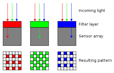
The most commonly used CFA is the Bayer filter mosaic as shown on Figure 54. The filter pattern is 50% green, 25% red and 25% blue. It should be noted that both various modifications of colours and arrangement and completely different technologies are available, such as colour co-site sampling or the Foveon X3 sensor.
3.4. Image processing
After the image acquisition with the image sensor, the image processing should be started. In computer vision systems there are some typical processing steps which generally cover the operation of the automotive cameras. In the following listing, which is based on [34], these steps are detailed complemented with the automotive specialities.
Pre-processing – Before a computer vision method can be applied to image data in order to extract some specific piece of information, it is usually necessary to process the data in order to assure that it satisfies certain assumptions implied by the method. Examples are
Re-sampling in order to assure that the image coordinate system is correct.
Noise reduction in order to assure that sensor noise does not introduce false information.
Contrast enhancement to assure that relevant information can be detected.
Scale space representation to enhance image structures at locally appropriate scales.
Feature extraction – Image features at various levels of complexity are extracted from the image data. Typical examples of such features are
Lines, edges. Primarily used in lane, road sign and object detection functions.
Localized interest points such as corners.
More complex features may be related to shape or motion.
Detection/segmentation – At some point in the processing a decision is made about which image points or regions of the image are relevant for further processing. Examples are
Segmentation of one or multiple image regions which contain a specific object of interest. Typically used in night vision to separate the ambient light sources from the vehicle lights.
High-level processing – At this step the input is typically a small set of data, for example a set of points or an image region which is assumed to contain a specific object. The remaining processing deals with, for example:
Verification that the data satisfy model-based and application specific assumptions.
Estimation of application specific parameters, such as object size, relative speed and distance.
Image recognition – classifying a detected object into different categories. (E.g. passenger vehicle, commercial vehicle, motorcycle.)
Image registration – comparing and combining two different views of the same object in stereo cameras.
Decision making – Making the final decision required for the application. These decisions can be classified as mentioned in Section 1.3, for example:
Inform about road sign
Warn of the lane departure
Support ACC with lanes, objects’ speed and distance (adding complementary information to the radar)
Intervene with steering or breaking in case of lane departure
3.5. Applications
The automotive cameras can be classified several ways. The most important aspects are the location (front, rear), colouring (monochrome, monochrome+1 colour, RGB) and the spatiality (mono, stereo).
The rear cameras are usually used for parking assistant functions, whilst the front cameras can provide several functions such as:
Object detection
Road sign recognition
Lane detection
Vehicle detection and environment sensing by dark for headlight control
Road surface quality measurement
Supporting and improve radar-based functions (Adaptive Cruise Control, Predictive Emergency Braking System, Forward Collision Warning)
Traffic jam assist, construction zone assist
The colouring capabilities influence the reliability and the precision of some camera functions. Basically most of the main functions can be implemented with a mono camera, which detects only the intensity of light on each pixel. On the other hand only one plus colour can significantly help to reach better performance. For example with red sensitive pixels the road sign recognition could be more reliable.
The mono or stereo design of the camera has strong influence on the 3D vision, which is important for measuring the distances of the objects and to detect the imperfections of the road.
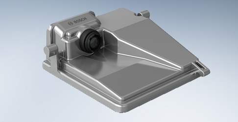
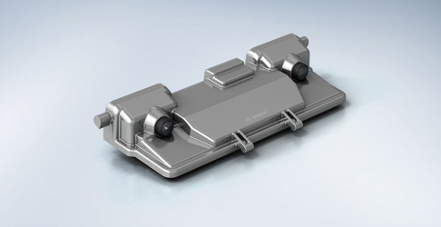
To deal with the aforementioned tasks the output of the imager is processed by a high computing performance CPU-based control unit. The CPU is often supported with an FPGA which is fast enough to perform the pre-processing and feature extraction tasks.
The output of the camera can be divided into two classes, which also means two different architectures:
Low-level (image) interfaces: analogue, LVDS (low-voltage differential signalling)
High-level (identified objects description): CAN, FlexRay
In the first case the imager with the lens and the control unit are installed in different places inside the vehicle, whilst in the second case all of the necessary parts are integrated into a common housing and placed beyond the windshield. This integrative approach doesn’t require a separate control unit.
As an example of a modern automotive camera the Stereo Video Camera of Bosch has the following main properties. Its two CMOS (complementary metal oxide semiconductor) colour imagers have a resolution of 1280 x 960 pixels. Using a powerful lens system, the camera records a horizontal field of view of 45 degrees and offers a 3D measurement range of more than 50 meters. The image sensors, which are highly sensitive in terms of lighting technology, can process very large contrasts and cover the wavelength range that is visible to humans.
This stereo camera enables a variety of functions that has already been mentioned before. The complete three-dimensional recording of the vehicle's surroundings also provides the basis for the automated driving functions of the future. (Source: [35]
Compared to the aforementioned Bosch Stereo Camera the following table shows the main properties of the Continental CSF200 mono camera.
Range | Maximum: 40m … 60m |
Sensor | RGB 740 x 480 pixel |
Field of view | horizontal coverage: 42° vertical coverage: 30° |
Cycle Time | 60ms |
3.6. Night Vision
The digital imaging and computer vision have become more and more important on the road towards the fully autonomous car. But the imagers in these cameras have got a hard constraint which is the absence of light. To overcome these shortcomings several night vision systems were developed in the past decades, which is summarized in the followings based on [36].
Nowadays there are two main technologies are available for the vehicle manufacturers:
Far Infrared (FIR) technology
Near Infrared (NIR) technology
An FIR system is passive, detecting the thermal radiation (wavelength of around 8–12 um). Warm objects emit more radiation in this region and thus have high visibility in the image. NIR systems use a near-infrared source to shine light with a wavelength of around 800 nm at the object and then detect the reflected illumination. The main advantage of NIR systems is that the cost is lower, because the sensor technology at these wavelengths is already well developed for other imaging applications such as video cameras. A NIR hardware can also potentially be combined with other useful functions such as lane departure warning.
In contrast, FIR systems offer a superior range and pedestrian-detection capability, but their sensors cannot be mounted behind the windscreen or other glass surfaces. University of Michigan Transport Research Institute studies comparing the ability of drivers to spot pedestrians using both the NIR and FIR devices showed that under identical conditions, the range of an FIR system was over three times further than that obtained with NIR — 119 m compared with 35 m.
Pros | NIR | Pros | FIR |
Lower sensor cost | Superior detection range | ||
Higher image resolution | Emphasizes objects of particular risk for example, pedestrians and animals | ||
Potential for integrating into other systems | Images with less visual clutter (unwanted features that may distract driver) | ||
Favourable mounting location | Better performance in inclement weather | ||
Cons | Cons | ||
Sensitive to glare from oncoming headlights and other NIR systems | Lower contrast for objects of ambient temperature | ||
Detection range depends on reflectivity of object |
|
Night-vision systems were first introduced into the 2000 model of the Cadillac Deville (FIR) and thereafter by Lexus/Toyota in 2002 (NIR). In September 2005, BMW introduced the Autoliv Night Vision System [37] as an optional feature which used a thermal image sensor. featuring a 320 times 240 array of detector elements (pixels) that sense very small temperature differences in the environment (less than a tenth of a degree). The sensor, 57 x 58 x 72 mm in size excluding the connector, is mounted on the car's front bumper just below and to one side of the number plate.
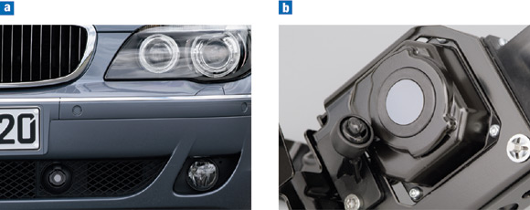
In terms of performance, the system offers a range of 300 m, a 36° field of view in the horizontal and a 30 Hz refresh rate. By using a highly sensitive FIR camera, the driver is given a clear view of the road ahead and can easily distinguish warm (living) objects that have a temperature different from that of the ambient air. For ease of use, the image is automatically optimized to preserve image quality over a range of driving conditions.

For driving speeds in excess of 70 km per hour, the image is automatically magnified 1.5 times using an electronic zoom function. An electronic panning function, which is controlled by the angle of the steering wheel, ensures that the image matches the car direction and follows the curve of the road.
3.7. Laser Scanner (LIDAR)
Similarly to RADAR LiDAR means LIght Detection And Ranging. The main purpose of the laser scanner system is the detection and tracking of other vehicles, pedestrians and stationary objects (e.g. guard rails).
Differences between Lidars and laser scanners are detailed in the following paragraphs. The Lidar is static which means it can measure in one direction (Traffipax). Instead of radio waves used by RADAR, LIDAR uses ultra violet, visible or infrared light pulses for detection. The light pulses are sent out of the sensor in many directions simultaneously and reflected by the surrounding objects. Object distance detection is based on precise time measurement of the pulse-echo reflection. Repeated measurement can result in speed detection of the measured object.
The Laser Scanner is dynamic which means variable viewing angle. As the LIDAR measurements are taken many times with a rotating sensor in many directions, the result is a scanned planar slice. This type of measurement is called Laser Scanning. If the measurements are taken also in different angles or the sensor is moving (on top of vehicle) a complete 3D view of the surroundings can be created.
As this process can be done many times a second (5-50Hz) a real time view of the surrounding can also be created. (Source [38]
The laser scanner may also provide lane markings detection. Together with the lane marking information of the front camera this additional feature might help to provide redundant and robust lane information.
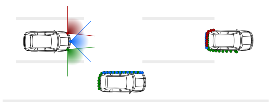
Figure 47 shows a typical laser scanner system consists of three single sensors integrated in the vehicles front bumper. One sensor is installed in the centre of the vehicle looking straight ahead. Two further sensors are integrated in the left and right front corner of the vehicle facing outwards at 30° to 40°. There is a sensor fusion algorithm that creates a complete 180 degree view to the front direction of the vehicle.
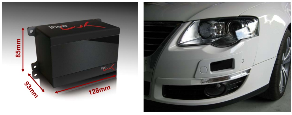
The ibeo LUX HD [39] laser scanner which is designed for reliable automotive ADAS applications and tested in project HAVEit has the following main properties.
Range up to 120m (30m @10% remisson)
All weather capability thanks to the Ibeo multi-echoe-technology: Up to 3 distance measurements per shot (allow measurements through atmospheric clutter like rain and dust)
Embedded object tracking
Wide horizontal field of view: 2 layers: 110° (50° to - 60°), 4 layers: 85° (35° to -50°)
Vertical field of view: 3.2°
Multi-layer: 4 parallel scanning layers
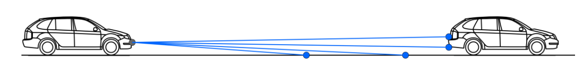
Data update rate: 12.5/ 25.0/ 50.0 Hz
Operating temperature range: -40 to 85 deg C
Accuracy (distance independent): 10 cm
Angular resolution:
Horizontal: up to 0.125°
Vertical: 0.8°
Distance Resolution: 4 cm
Another important product is the Velodyne HDL-64E S2 [40] laser scanner. It is designed for obstacle detection and navigation of autonomous ground vehicles and marine vessels. Its durability, 360° field of view and very high data rate makes this sensor ideal for the most demanding perception applications as well as 3D mobile data collection and mapping applications. This laser scanner is used in Google’s driverless car project.
905 nm wavelength, 5 ns pulses
15V 4A
Ethernet output
less than 2 cm accuracy
Max 15 Hz update rate (900RPM)
Range 120m
0.09 degree of vertical resolution
26 degree of vertical field of view
More than 1.3 million points detected per second
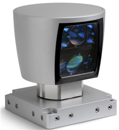
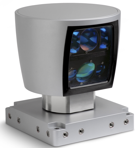
Typical components of a laser scanner sensor are the following:
Laser source (emitters)
Scanner optics
Laser detector (receivers)
Control electronics
Position and navigation systems
The general architecture of the laser scanners is shown in Figure 51.
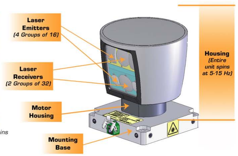
Should the horizontal aperture angle be not enough for a specific application that requires a greater field of vision, there is fusion scan available. Up to six sensors can be combined together. The data of the individual sensors are synchronized and combined together using a special software, resulting in one fused scan. With laser scanner fusion there is a possibility to achieve a seamless 360 degrees scanning of the vehicle's surroundings.
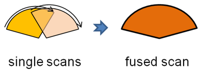
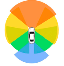
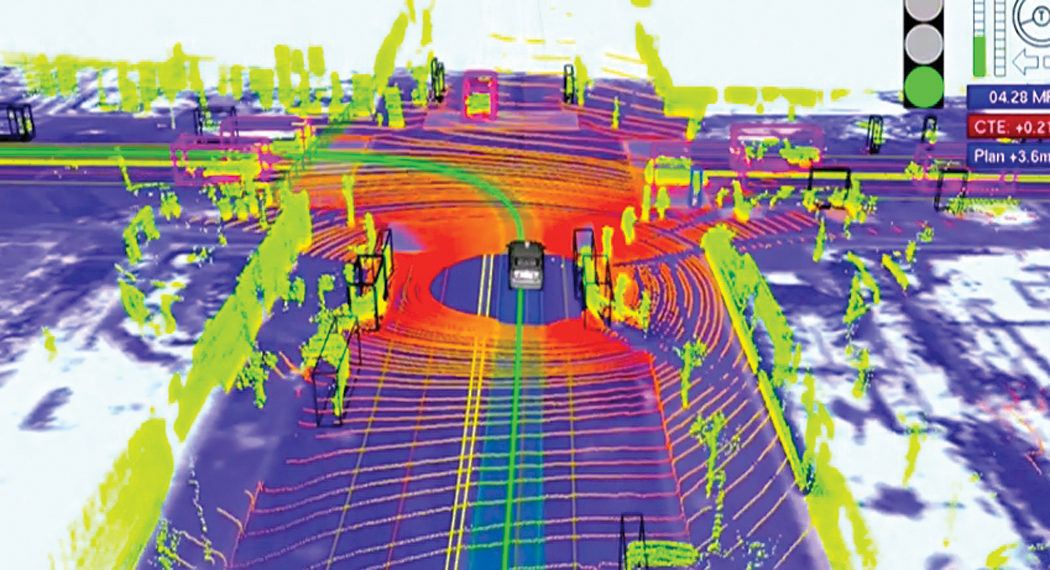
3.8. eHorizon
The so-called eHorizon is an integrated information source including map information, route information, speed limit information, 3D landscape data, positioning and navigation information (GPS, GLONASS, etc.) for the advanced driver assistance systems (ADAS) within the car. With the help of this information the forward thinking driving function can be improved (e.g. predictive control considering road inclinations and speed limits) and the fuel consumption can be decreased.
3.8.1. NAVSTAR GPS
The Navigation Signal Timing and Ranging Global Positioning System (NAVSTAR GPS, in short GPS) is a U.S. government owned utility that provides users with positioning, navigation, and timing (PNT) services. The following summary of the operating principles is based on [41].
This system consists of three segments: the space segment, the control segment, and the user segment. The U.S. Air Force develops, maintains, and operates the space and control segments.
The space segment consists of a constellation of satellites transmitting radio signals to users. The United States is committed to maintaining the availability of at least 24 operational GPS satellites, 95% of the time. To ensure this commitment, the Air Force has been flying 31 operational GPS satellites for the past few years. The extra satellites may increase GPS performance but are not considered part of the core constellation. GPS satellites fly in medium Earth orbit (MEO) at an altitude of approximately 20,200 km. Each satellite circles the Earth twice a day. The satellites in the GPS constellation are arranged into six equally-spaced orbital planes surrounding the Earth. Each plane contains four "slots" occupied by baseline satellites. This 24-slot arrangement ensures users can view at least four satellites from virtually any point on the planet.
The control segment consists of a global network of ground facilities that track the GPS satellites, monitor their transmissions, perform analyses, and send commands and data to the constellation. The current operational control segment includes a master control station, an alternate master control station, 12 command and control antennas, and 16 monitoring sites.
The user segment consists of the GPS receiver equipment, which receives the signals from the GPS satellites and uses the transmitted information to calculate the user’s three dimensional position and time.
The GPS satellites broadcast radio signals providing their locations, status, and precise time (t1) from on-board atomic clocks.
The principle of the operation is based on distance measurement. The GPS satellites broadcast radio signals providing their locations, status, and precise time from on-board atomic clocks. The GPS radio signals travel through space at the speed of light. A GPS device receives the radio signals, noting their exact time of arrival, and uses these to calculate its distance from each satellite in view. To calculate its distance from a satellite, a GPS device applies this formula to the satellite's signal:
distance = rate x time
where rate is the speed of light and time is how long the signal travelled through space
(This requires quite precise time measurement, since 1 us time deviation would result in 300m distance deviation.) The signal's travel time is the difference between the time broadcast by the satellite and the time the signal is received.
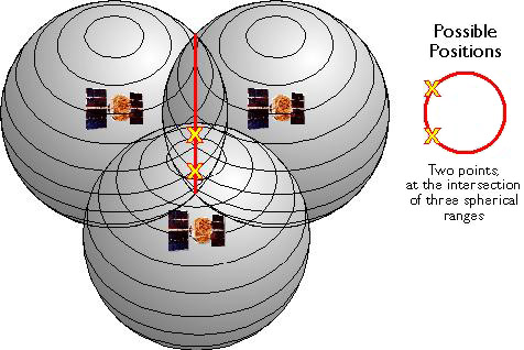
If distances from three satellites are known, the receiver's position must be one of two points at the intersection of three spherical ranges (see Figure 54). GPS receivers are usually smart enough to choose the location nearest to the Earth's surface. At a minimum, three satellites are required for a two-dimensional (horizontal) fix if our receiver’s clock would be perfect. In this theoretical case all our satellite ranges would intersect at a single point (which is our position). But with imperfect clocks, a fourth measurement, done as a cross-check, will not intersect with the first three. Since any offset from universal time will affect all of our measurements, the receiver looks for a single correction factor that it can subtract from all its timing measurements that would cause them all to intersect at a single point. That correction brings the receiver's clock back into sync with universal time. Once it has that correction it applies to all the rest of its measurements and now we've got precise positioning. One consequence of this principle is that any decent GPS receiver will need to have at least four channels so that it can make the four measurements simultaneously.
The modernization program of the GPS was started in May 2000 with turning off the GPS Selective Availability (SA) feature. SA was an intentional degradation of civilian GPS accuracy, implemented on a global basis through the GPS satellites. During the 1990s, civil GPS readings could be incorrect by as much as a football field (100 meters). On the day SA was deactivated, civil GPS accuracy improved tenfold, benefiting civil and commercial users worldwide. In 2007, the government announced plans to permanently eliminate SA by building the GPS III satellites without it. The GPS modernization program involves a series of consecutive satellite acquisitions. It also involves improvements to the GPS control segment, including the Architecture Evolution Plan (AEP) and the Next Generation Operational Control System (OCX). The main goal is to improve GPS performance using new civilian and military signals. In addition GPS modernization is introducing modern technologies throughout the space and control segments that will enhance overall performance. For example, legacy computers and communications systems are being replaced with a network-centric architecture, allowing more frequent and precise satellite commands that will improve accuracy for everyone.
From the point of view of the transportation the Second and the Third Civil Signals (L2C and L5) will be the most significant changes in the modernized GPS system. L2C is designed specifically to meet commercial needs. When combined with L1 C/A in a dual-frequency receiver, L2C enables ionospheric correction, a technique that boosts accuracy. Civilians with dual-frequency GPS receivers enjoy the same accuracy as the military (or better). For professional users with existing dual-frequency operations, L2C delivers faster signal acquisition, enhanced reliability, and greater operating range. L2C broadcasts at a higher effective power than the legacy L1 C/A signal, making it easier to receive under trees and even indoors.
L5 is designed to meet demanding requirements for safety-of-life transportation and other high-performance applications. L5 is broadcast in a radio band reserved exclusively for aviation safety services. It features higher power, greater bandwidth, and an advanced signal design. Future aircraft will use L5 in combination with L1 C/A to improve accuracy (via ionospheric correction) and robustness (via signal redundancy). In addition to enhancing safety, L5 use will increase capacity and fuel efficiency within U.S. airspace, railroads, waterways, and highways.
Both signals are in launching phase. The L2C will be available on 24 GPS satellites around 2018 and the L5 around 2021.
3.8.2. GLONASS
GLONASS (Globalnaya Navigatsionnaya Sputnikovaya Sistema or Global Navigation Satellite System) is a GNSS operated by the Russian Aerospace Defence Forces. Development of GLONASS began in 1976, with a goal of global coverage by 1991 [42]. Beginning on 12 October 1982, numerous rocket launches added satellites to the system until the constellation was completed in 1995. GLONASS was developed to provide real-time position and velocity determination, initially for use by the Soviet military in navigating and ballistic missile targeting. With the collapse of the Russian economy GLONASS rapidly degraded, mainly due to the relatively short design life-time of the GLONASS satellites. Beginning in 2001, Russia committed to restoring the system, and in recent years has diversified, introducing the Indian government as a partner. This plan calls for 18 operational satellites in orbit by 2008 and 24 satellites (21 operational and 3 on-orbit spares deployed in three orbital planes) in place by 2009; and a level of performance matching that of the U.S Global Positioning System by 2011. Finally by 2010, GLONASS has achieved 100% coverage of Russia's territory and in October 2011, the full orbital constellation of 24 satellites was restored, enabling full global coverage. It both complements and provides an alternative to the United States' Global Positioning System (GPS) and is the only alternative navigational system in operation with global coverage and of comparable precision.
At present GLONASS provides real time position and velocity determination for military and civilian users. The fully operational GLONASS constellation consists of 24 satellites, with 21 used for transmitting signals and three for in-orbit spares, deployed in three orbital planes. The three orbital planes' ascending nodes are separated by 120° with each plane containing eight equally spaced satellites. The orbits are roughly circular, with an inclination of about 64.8°, and orbit the Earth at an altitude of 19,100 km, which yields an orbital period of approximately 11 hours, 15 minutes. The planes themselves have a latitude displacement of 15°, which results in the satellites crossing the equator one at a time, instead of three at once. The overall arrangement is such that, if the constellation is fully populated, a minimum of 5 satellites are in view from any given point at any given time. This guarantees for continuous and global navigation for users world-wide.
3.8.3. Galileo
Galileo is Europe’s own global navigation satellite system, providing a highly accurate, guaranteed global positioning service under civilian control, which is introduced from [43].
By offering dual frequencies as standard, Galileo will deliver real-time positioning accuracy down to the metre range. It will guarantee availability of the service under all but the most extreme circumstances and will inform users within seconds of any satellite failure, making it suitable for safety-critical applications such as guiding cars, running trains and landing aircraft. On 21 October 2011 came the first two of four operational satellites designed to validate the Galileo concept in both space and on Earth. Two more followed on 12 October 2012. This In-Orbit Validation (IOV) phase is now being followed by additional satellite launches to reach Initial Operational Capability (IOC) by mid-decade.
Galileo services will come with quality and integrity guarantees, which mark the key difference of this first complete civil positioning system from the military systems that have come before. A range of services will be extended as the system is built up from IOC to reach the Full Operational Capability (FOC) by this decade’s end. The fully deployed Galileo system consists of 30 satellites (27 operational + 3 active spares), positioned in three circular Medium Earth Orbit (MEO) planes at 23 222 km altitude above the Earth, and at an inclination of the orbital planes of 56 degrees to the equator.
The four operational satellites launched so far - the basic minimum for satellite navigation in principle - serve to validate the Galileo concept with both segments: space and related ground infrastructure. On March 12th, 2013, a first positioning test based on the 4 first operational Galileo satellites was conducted by ESA. This first position fix returned an accuracy range of +/- 10 meters, which is considered as very good, considering that only 4 satellites (out of the total constellation of 30) are already deployed. The Open Service, Search and Rescue and Public Regulated Service will be available with initial performances soon. Then as the constellation is built-up beyond that, new services will be tested and made available to reach Full Operational Capability (FOC). Once this is achieved, the Galileo navigation signals will provide good coverage even at latitudes up to 75 degrees north, which corresponds to Norway's North Cape - the most northerly tip of Europe - and beyond. The large number of satellites together with the carefully-optimised constellation design, plus the availability of the three active spare satellites, will ensure that the loss of one satellite has no discernible effect on the user.
3.8.4. BeoiDou (COMPASS)
The BeiDou Navigation Satellite System (BDS) is a Chinese satellite navigation system. It consists of two separate satellite constellations – a limited test system that has been operating since 2000, and a full-scale global navigation system that is currently under construction.
The first BeiDou system, officially called the BeiDou Satellite Navigation Experimental System and also known as BeiDou-1, consists of three satellites and offers limited coverage and applications. It has been offering navigation services, mainly for customers in China and neighbouring regions, since 2000.
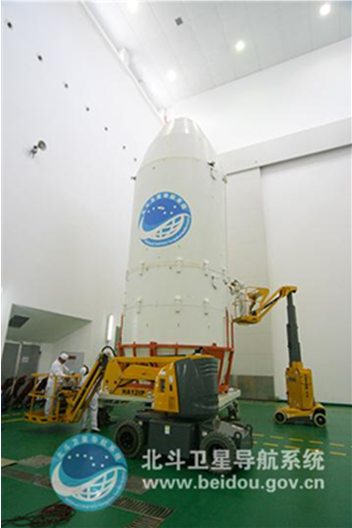
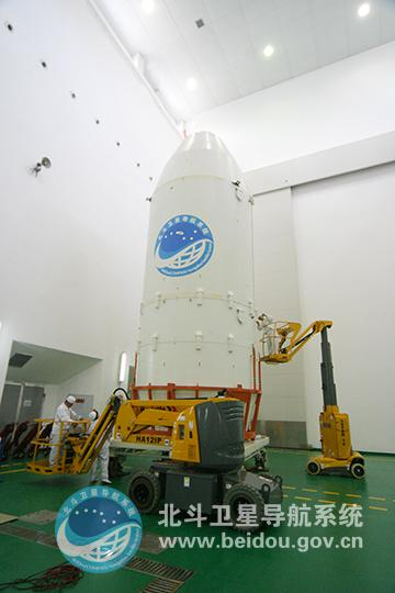
The second generation of the system officially called the BeiDou Satellite Navigation System (BDSNS) and also known as COMPASS or BeiDou-2, will be a global satellite navigation system. According to the plans the full constellation will consist of 35 satellites. Since December 2012 there are 10 satellites providing local services to the Asia-Pacific area and it is planned to cover all over the world serving global customers before 2020. [44]
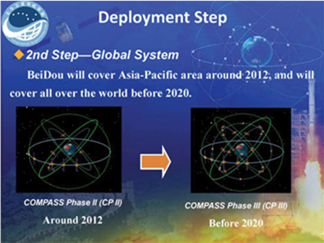

The COMPASS Phase II has successfully established as planned. On December 27, 2013, the first anniversary of BeiDou Navigation Satellite System providing full operational regional service was held in Beijing. At the meeting, China Satellite Navigation System Management Office Director Ran Chengqi announced the BeiDou Navigation Satellite System Public Service Performance Standard.
The result comparison with GPS created by John Lavrakas (Advanced Research Corporation) [45] shows mixed results. In some cases, the commitments from BeiDou were stronger (URE accuracy, the table to show green for the GNSS service committing to a more stringent standard over the other vertical position), and in other cases the commitments from GPS were stronger (continuity of service, advance notice of outages).
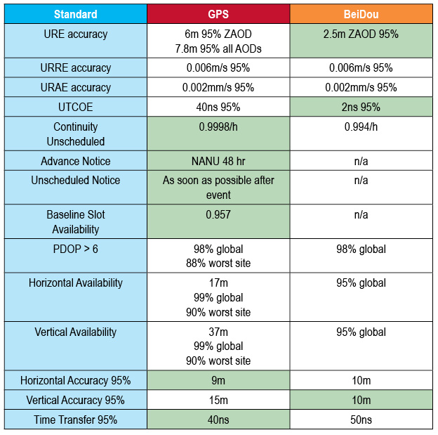
3.8.5. Differential GPS
Differential correction techniques are used to enhance the quality of location data gathered using global positioning system (GPS) receivers. Differential correction can be applied either in real-time (directly in the field, during measurement) or when post-processing data in the office (later during data evaluation). Although both methods are based on the same underlying principles, each accesses different data sources and achieves different levels of accuracy. Combining both methods provides flexibility during data collection and improves data integrity.
The underlying assumption of differential GPS (DGPS) technology is that any two receivers that are relatively close together will experience similar atmospheric errors. DGPS requires that one GPS receiver must be set up on a precisely known location. This GPS receiver is the base or reference station. The base station receiver calculates its position based on satellite signals and compares this location to the already known precise location resulting in a difference. This difference then is applied to the GPS data recorded by the second GPS receiver, which is known as the roving receiver. The corrected information can be applied to data from the roving receiver in real time in the field using radio signals or through post-processing after data capture using special processing software.
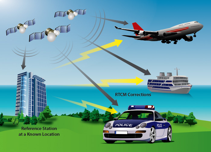
Real-time DGPS occurs when the base station calculates and broadcasts corrections for each satellite as it receives the data. The correction is received by the roving receiver via a radio signal if the source is land based or via a satellite signal if it is satellite based and applied to the position it is calculating. As a result, the position displayed and logged to the data file of the roving GPS receiver is a differentially corrected position.
In the US, the most widely available DGPS system is the Wide Area Augmentation System (WAAS). The WAAS was created by the Federal Aviation Administration and the Department of Transportation for use in precision flight approaches. However, the system is not limited to aviation applications, and many of the commercial GPS receivers intended for maritime and automotive use support WAAS. WAAS provides GPS correction data across North America with a typical accuracy less than 5 meters. Similar systems are available in Europe.
The European Geostationary Navigation Overlay Service (EGNOS) is the first pan-European satellite navigation system. It augments the US GPS satellite navigation system and makes it suitable for safety critical applications such as flying aircraft or navigating ships through narrow channels.
Consisting of three geostationary satellites and a network of ground stations, EGNOS achieves its aim by transmitting a signal containing information on the reliability and accuracy of the positioning signals sent out by GPS. It allows users in Europe and beyond to determine their position to within 1.5 meters. (Source: [46])
Another high precision GPS solution is the real-time kinematic GPS (RTK GPS). RTK is a GBS-based survey that utilizes a fixed, nearby ground base station that is in direct communication with the rover receiver through a radio link. RTK is capable of taking survey grade measurements in real time and providing immediate accuracy to within 1-5 cm. RTK systems are the most precise of all GNSS systems. They are also the only systems that can achieve complete repeatability, allowing the returning to the exact location indefinitely. All this precision and repeatability comes at a fairly high cost. But there are other drawbacks to RTK also. RTK requires a base station within about 10-15 km of the rover. [47]
3.8.6. Assisted GPS
Assisted GPS describes a system where outside sources, such as an assistance server and reference network, help a GPS receiver perform the tasks required to make range measurements and position solutions. The assistance server has the ability to access information from the reference network and also has computing power far beyond that of the GPS receiver. The assistance server communicates with the GPS receiver via a wireless link (generally mobile network data link). With assistance from the network, the receiver can operate (start-up) more quickly and efficiently than it would unassisted, because a set of tasks that it would normally handle is shared with the assistance server. The resulting AGPS system, consisting of the integrated GPS receiver and network components, boosts performance beyond that of the same receiver in a stand-alone mode. It improves the start-up performance or time-to-first-fix (TTFF) of the GPS receiver. The assistance server is also able to compute position solutions, leaving the GPS receiver with the sole job of collecting range measurements. The only disadvantage of AGPS is that it depends on the infrastructure (requiring an assistant service and an on-line data connection). (Source: [48])
3.9. Data Fusion
The data fusion is responsible for comparing all relevant sensor information, carrying out feasibility increasing the reliability of the individual sensor information and increasing precision of the sensor information. The data fusion provides all necessary information to the following command layer in order to be able to complete its task successfully.
The Data Fusion harmonizes the on-board environment sensor signal, the vehicle sensor signals (vehicle speed, yaw rate, steering angle, longitudinal, lateral acceleration, etc.) The output of the sensor fusion is the vehicle status (Position and kinematic state information); and environmental status (position and shape of the surrounding objects including the vehicle in front of us). The environmental objects can also be classified into categories be means of dimension and type of objects.
Front vehicle
Surrounding objects (obstacles)
Lane information
Road information
Intersection information
Trip information
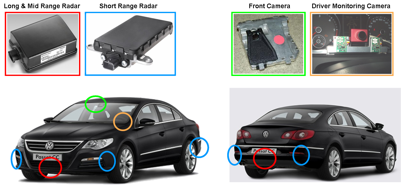
Sensor data fusion calculates an overall environment perception taking the information of all sensors into account.
Sensor data fusion is generally a separate module inside the vehicle control system. It receives data from many sources, including in-vehicle sensors, environment monitoring sensors (radar, laser and camera), V2V communication, eHorizon, etc. The environment sensors are heterogeneous sources of information, providing data describing surrounding objects and road. Each sensor makes different estimates of the environment properties, using both overlapping and independent fields of view. Moreover, each of these sources transmits data in its own spatial and temporal format.
The sensor data fusion gathers sensor data and executes several tasks in order to provide useful estimates which are synchronized and spatially aligned. The synchronised and spatially aligned data, called the perception model, is then available for Highly Automated Driving applications. The perception model consists of state estimations of relevant objects, the road and a refined ego vehicle state.
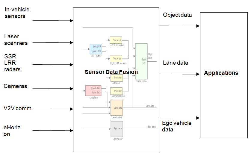
To achieve the synchronized and spatially aligned view of the environment, the sensor data fusion will make use of several algorithms and filters to provide high level output data.
There are several sensors measuring the same objects surrounding the vehicle (laser scanners, short and long range radars, mono and colour cameras, V2V communication). Each sensor measures different aspects of an object, for example, the laser scanners measure both position and velocity, whereas the camera simply estimates object position. Therefore each sensor data have to be evaluated and filtered first to reach a common (homogenous) object representation, then comes the effective fusion of the data.
There are several algorithms exist for sensor data fusion, such as Cross-Covariance Fusion, Information Fusion, Maximum A-Posterior Fusion and Covariance Fusion.
The standardized output state for each detected object contains the following information:
Position
Vehicle Speed and Acceleration)
Object Size
Object Classification (tree, vehicle, pedestrian, etc.)
Output Data Confidence Level
Chapter 4. Human-Machine Interface
The Human-Machine Interfaces specifies the bidirectional connection from the driver to the vehicle. Designing a good HMI device is a challenging engineering task. Creation of a well-operable, user-friendly and ergonomic interface presumes great expertise.
In this Chapter the requirements of automotive HMIs, the classification and its technologies are detailed.
4.1. Requirements
The general requirements of the automotive HMIs can be summarized as follows. The HMI should inform and support the intervention considering the following aspects:
Readability
Clarity
Interpretability
Accessibility
Ease of handling
The above mentioned requirements aim to increase the traffic safety. All of these points serve that the handling of the vehicle should not distract the driver.
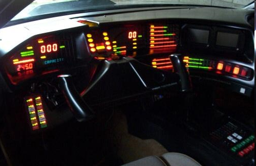
Today, a wide range of new in-vehicle technologies exist, which are introduced in this lecture, such as Advanced Driver Assistance Systems (ADAS) and In-vehicle Information Systems (IVIS). Moreover, the number of in-vehicle use of portable computing devices is increasing rapidly. These new technologies have great potential for enhancing road safety, as well as enhancing the quality of life and work, e.g. by providing in-vehicle access to new information and communication resources. However, the safety benefits of ADAS may be significantly reduced, or even cancelled, by unexpected behavioural responses to the technologies, e.g. system over-reliance and safety margin compensation. Moreover, IVIS and portable devices may induce dangerous levels of workload and driver distraction.
These problems and challenges have called to life the AIDE (Adaptive Integrated Driver-vehicle Interface) pan-European project. The general goal of the AIDE Integrated Project is to generate the knowledge and develop methodologies and human-machine interface technologies required for safe and efficient integration of ADAS, IVIS and portable devices into the driving environment. (Source: [49])
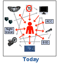

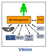
The basic theory behind AIDE can be summarized as follows. The term driver coaching involves “standard” HMI aspects and components such as visual/manual interactions with an application via a display and input controls. If a driver coaching application wants to transmit information to the driver (e.g. a pop-up message on a display), this presentation should be coordinated with other applications. If the driver is interacting with the coaching application, suppressing information from other in-vehicle applications during this interaction might be preferable. An additional possibility could be implementing the adaptivity of applications to the Driver-Vehicle-Environment (DVE) state by avoiding to provide low priority information when the driver workload is high, e.g. due to the traffic situation. (Source: [50])
As an HMI design example, in the HAVEit project, the control of the Human Machine Interface (HMI) is implemented in the command layer. The HMI control triggers the pop-ups that should be shown to the driver and decides which one to show from a prioritisation of all available pop-ups. All timing of the pop-ups is situated and parameterized in the HMI control.
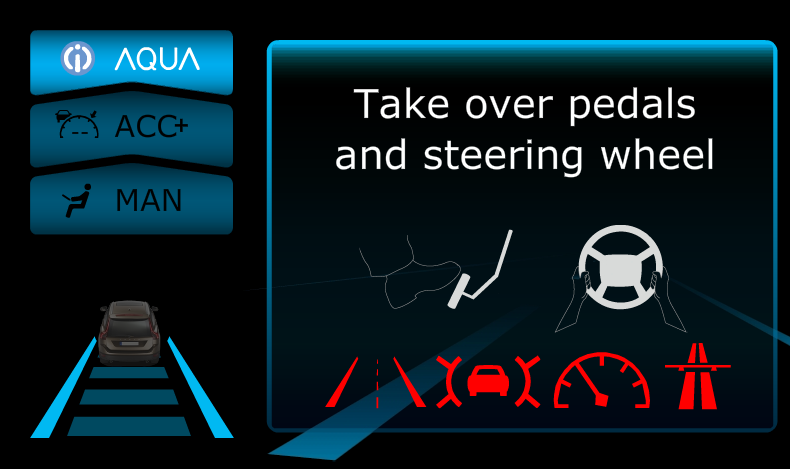
4.2. HMI classifications
The automotive HMIs can be classified in several ways. Our classifications detailed in the next sections are based on the relevance, the direction (I/O) and the applied technology of the HMIs.
The direction parameter can be input or output from the drivers’ point of view. While through the input interfaces the driver can intervene into the operation of the vehicle, the output interfaces enable the indication of any vehicle parameter, thus notifying the driver about any information.
In the following subsections the relevance groups are detailed. The technical solutions are especially various and diverse, hence the authors considered the detailed explanation important. That is why the applied technologies are described in a new section.
4.2.1. Primary HMI components
The primary HMI components are used for operating the vehicle basic functions and let the driver control the movement of the vehicle. Furthermore some of these components (and the minimum set of the devices) are regulated by the legal authorities. The following primary components can be considered as a basic primary HMI set in a passenger car with manual gearbox:
Input devices
Steering wheel
Pedals (accelerator, brake, clutch)
Gear shift lever
Parking brake
Turn indicator stalk
Wiper stalk
Light switch
Horn
Output devices
Instrument cluster
Speedometer
Important warning lights (oil pressure, charging etc.)
Turn signal indicator light
Fuel level
4.2.1.1. Input channels
It is important to explain the evolutionary process of the steering wheel and the accelerator and brake pedals. (The clutch and gear shift evolved in another way, because of the automatic gear shift systems.) Nowadays the x-by-wire systems are increasingly coming to the fore as mentioned in the Section “Intelligent Actuators”. The necessary technical solutions are available, “only” the responsibility and legal questions are not solved yet.
With using solely x-by-wire systems in case of the primary input HMIs, the connections to the actuators are electronic signals or high-level digital messages, which determine the desired motion state of the vehicle. This digital byte stream is often referred to as motion vector. It contains the demanded values for engine torque, brake pressure and steering angle and is extended by further values like gear-shift command. With this indirect connection, the electronic control units can execute the drivers command in a more effective and safer way.
In this technical level the input devices could be any type of human interfaces, the only requirement is to generate the proper electronic output. Beyond the conventional controls, several other possibilities are available, such as a joystick that is (besides the computer games) generally used to control forklifts. Although joysticks are technically perfectly integrated control devices, these solutions are not likely to be widespread in passenger cars, because they require absolute different driving techniques. Undoubtly x-by-wire systems have got a greater importance beyond the already utilized opportunities, namely the capability to control the vehicle by a computer. As the electronic interface (motion vector) can either be generated from the human driver or from an electronic control, the intelligent actuators cannot make a difference if the request was originated from driver or a control ECU. Moreover it is one of the basis of the highly automated or fully autonomous vehicle operation.
In modern vehicles the primary controls are equipped with several sensors which could be the following:
Steering wheel
Angle
Force, torque
Touching pressure and position (for detecting the driver presence and state)
Driver pulse detection for medical purposes
Pedals
Position
Force
Gear shift lever
Reverse detection
Position detection
4.2.1.2. Output channels
The primary HMI output is the instrument cluster. Basically it is responsible for displaying the motion state of the vehicle and the engine (such as velocity and rotational speed), feedback about the execution of the desired task (such as turn signal indicator light), and warning of the problems and errors. Additionally it could inform the driver about the detailed vehicle status, the driving situation and the current level of automation.
If we look through the evolution of the instrument cluster, it can be noticed that the development direction goes from the mechanical to the fully electronic solutions. Until the 1990s the analogue gauge of the speedometer was connected to the gearbox by a Bowden cable. Initial electric gauges used Deprez instruments, later they were driven by PWM signals using cross-coils technology. With release of the electronic motor control units, the needle of the gauge was driven by a small stepper motor which connected to the ECM. The instrument cluster has been complemented with alphanumeric and later graphical LCD displays. Nowadays the state-of-art solution is the fully colour LCD-based instrument cluster with variable style displaying. These technologies will be detailed in Section 4.3.
4.2.2. Secondary HMI components
The role of the secondary HMI components is to operate and display the comfort and infotainment functions. The controls can be found on the dashboard, around the central armrest, on the door armrest, on the steering wheel and sometimes over the central mirror. Naturally nowadays it is a very diverse and large component group. The size and content is highly dependent on the equipment features of the vehicle. Basically it contains the control inputs of the heating, ventilation, and air conditioning (HVAC) system and the radio, and some indicator lights and alphanumeric LCDs.
4.2.2.1. Input channels
The evolution of the secondary input controls is very diverse, but it has a common property at each manufacturer, namely the multiplication of the comfort and infotainment functions. It has resulted many buttons, switches, sliders and knobs all around the driver. The first solutions for the simplification were the integrated controllers with which the driver can navigate through a menu on an LCD display.
The BMW iDrive Controller was designed to be one single interface for many functions and features of the vehicle through the central console display, as replacing the array of controls of the comfort and infotainment functions with an all-in-one unit. The rotate-and-press mechanism enables one-handed operation: right means ‘continue’, left ‘back’, turning the button allows you to scroll through a list and pressing it selects an option. Frequently used functions like multimedia, radio or navigation have direct access keys. (Source: [51])
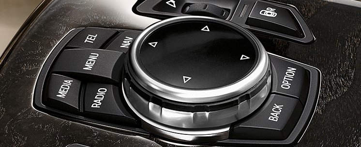
Several other methods exist to simplify the secondary input HMIs, such as steering wheel buttons and touchscreens. Generally most of these solutions are based on a menu, displayed on a relatively large screen.
The design of the secondary input devices is a more and more challenging task, because of the conflicting requirements, i.e. the increasing number of functions (especially infotainment) and the traffic safety.
4.2.2.2. Output channels
The secondary HMI output channels do not differ that much from the primary output channels, meaning that they are mostly relatively big LCD displays, but they may include special features like touch-screen control or split view of the central console, where on the same display device the driver and the “navigator” views different pictures at the same time.
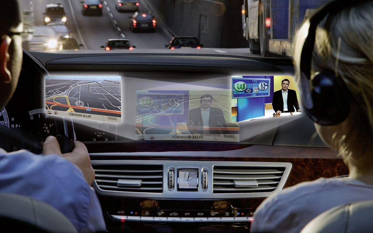
4.3. HMI technologies
In the following subsections the main groups of the applied HMI technologies are detailed.
4.3.1. Mechanical interfaces
In this subsection the mechanical interfaces are introduced. We classified those technologies into this group, which require mechanical impact from the driver, which could be the following:
Press by hand, finger or foot
Pull, slide or rotate by hand
Touch by hand or finger
4.3.1.1. Pedal, lever
Beside the steering wheel the pedals are the basic primary inputs in an automobile. As mentioned in the earlier sections electronic throttle control solutions are commonly used in today’s road vehicles.. The driver feeling of the “traditional” accelerator pedal can be substituted with a simple spring, because it requires only a constant pressure force. Furthermore the electronic pedal gives the possibility to use haptic feedback, such as vibration or variable pedal force to support the economic driving.
In conventional passenger cars the brake pedal is connected to the brake system via a rod in the hydraulic cylinder. Brake-by-wire systems are increasingly being integrated into or replacing conventional hydraulic or pneumatic brake systems. Such electrical brake systems are preferable because they reduce the mass of the system and provide greater ability to integrate the system into the vehicle's other electronic circuits and controls. In hybrid cars it is essential because of the electronic braking by the driving motor. During depression of the brake pedal in a conventional hydraulic braking system, the hydraulic fluid will exert a force back on the brake pedal due to the hydraulic pressure in the brake lines. Since an electronic brake system may not have such hydraulic pressure at the brake pedal, the vehicle operator will not detect any countering force, which in turn can disorient the operator. Accordingly, a typical electrical brake system will include a brake pedal feel simulator to provide a simulation force on the brake pedal. The simulation force provided by the simulator acts opposite the brake pedal force generated by the vehicle driver. It has to be noted that the brake pedal simulator has to suit to the different driving situations especially during emergency. The system has to adjust automatically its operation to reduce or eliminate the simulation force during emergency or failure conditions. (Source: [52])
The clutch pedal is usually hydraulic also, and exists only in vehicles with manual gearbox. It doesn’t require such developments as mentioned above, because with the use of automatic, automated or semi-automatic gearboxes the clutch pedal itself is eliminated.
Traditionally one mechanical lever exists in vehicles, i.e. the parking brake lever. In European vehicle designs it is operated by hand (hand-brake) but in the US the parking brake is generally operated by the left foot. In modern vehicle the parking brake lever is often substituted by a push button or a fully automatic parking brake.
4.3.1.2. Steering wheel
The steer-by-wire system (mentioned in Section “Intelligent actuators”) is also an enabler of good haptic HMI systems as it provides as much design freedom as possible, because the characteristics of the steering wheel are dynamically independent from the front axle steering. For example, a vibration induced in the steering wheel for warning purposes in a mechanically decoupled steer-by-wire systems can be designed with no effect on the actual steering behaviour at the front wheels.
4.3.1.3. Button, switch, stalk, slider
With the help of these components the driver can activate/deactivate or set the vehicle’s primary and secondary functions. These switching components could be single buttons or switches for each function, a stalk or a slider.
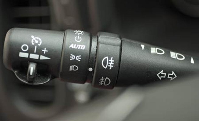
4.3.1.4. Integrated controller knob
The integrated controller knobs are such input devices which integrate more input functions into one device to support the much easier and more intuitive handling of the vehicle. These input functions could be rotation, push/pull and 4-way joystick.
A typical example is the BMW iDrive as mentioned in Section Input channels4.2.2.1, but a lot of simpler utilizations exist, such HVAC and radio control knobs.
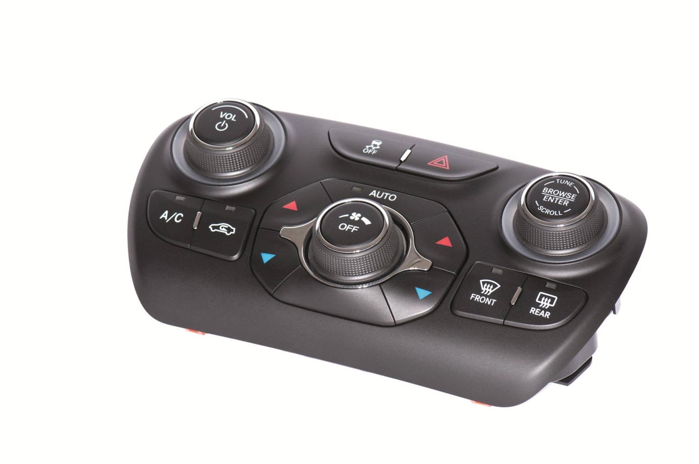
4.3.1.5. Touchscreen
Infotainment displays often have touchscreen features enabling the driver to select functions via touching the display. Touchscreen technology is the direct manipulation type gesture based technology. A touchscreen is an electronic visual display capable of detecting and locating a touch over its display area. It is sensitive to the touch of a human finger, hand, pointed finger nail and passive objects like stylus. Users can simply move things on the screen, scroll them, zoom them and many more.
There are four main touchscreen technologies:
Resistive
Capacitive
Surface Acoustic Wave
Infrared
The most wide-spread ones are the resistive and the capacitive touchscreens, thus these types will be detailed in the following paragraphs.
Resistive LCD touchscreen monitors rely on a touch overlay, which is composed of a flexible top layer and a rigid bottom layer separated by insulating dots, attached to a touchscreen controller. The inside surface of each of the two layers is coated with a transparent metal oxide coating (ITO) that facilitates a gradient across each layer when voltage is applied. Pressing the flexible top sheet creates electrical contact between the resistive layers, producing a switch closing in the circuit. The control electronics alternate voltage between the layers and pass the resulting X and Y touch coordinates to the touchscreen controller. The touchscreen controller data is then passed on to the computer operating system for processing.
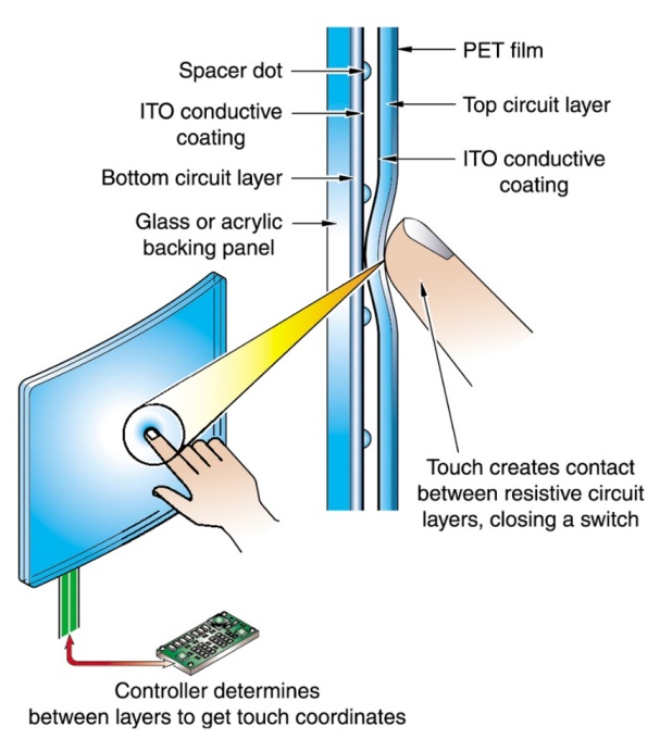
Because of its versatility and cost-effectiveness, resistive touchscreen technology is the touch technology of choice for many markets and applications. Resistive touchscreens are used in food service, retail point-of-sale (POS), medical monitoring devices, industrial process control and instrumentation, portable and handheld products. Resistive touchscreen technology possesses many advantages over other alternative touchscreen technologies (acoustic wave, capacitive, infrared). Highly durable, resistive touchscreens are less susceptible to contaminants that easily infect acoustic wave touchscreens. In addition, resistive touchscreens are less sensitive to the effects of severe scratches that would incapacitate capacitive touchscreens. Drawback can be the too soft feeling when pressing it, since there is a mechanical deformation required to connect the two resistive layers to each-other. (Source: [53])
One can use anything on a resistive touchscreen to make the touch interface work; a gloved finger, a fingernail, a stylus device – anything that creates enough pressure on the point of impact will activate the mechanism and the touch will be registered. For this reason, resistive touchscreen require slight pressure in order to register the touch, and are not always as quick to respond as capacitive touchscreens. In addition, the resistive touchscreen’s multiple layers cause the display to be less sharp, with lower contrast than we might see on capacitive screens. While most resistive screens don’t allow for multi-touch gestures such as pinch to zoom, they can register a touch by one finger when another finger is already touching a different location on the screen. (Source: [54])
The capacitive touchscreen technology is the most popular and durable touchscreen technology used all over the world. It consists of a glass panel coated with a capacitive (conductive) material Indium Tin Oxide (ITO). The capacitive systems transmit almost 90% of light from the monitor. In case of surface-capacitive screens, only one side of the insulator is coated with a conducting layer. While the screen is operational, a uniform electrostatic field is formed over the conductive layer. Whenever, a human finger touches the screen, conduction of electric charges occurs over the uncoated layer which results in the formation of a dynamic capacitor. The controller then detects the position of touch by measuring the change in capacitance at the four corners of the screen. In the projected-capacitive touchscreen technology, the conductive ITO layer is etched to form a grid of multiple horizontal and vertical electrodes. It involves sensing along both the X and Y axis using clearly etched ITO pattern. The projective screen contains a sensor at every intersection of the row and column, thereby increasing the accuracy of the system. (Source: [55])
Since capacitive screens are made of one main layer, which is constantly getting thinner as technology advances, these screens are not only more sensitive and accurate, the display itself can be much sharper. Capacitive touchscreens can also make use of multi-touch gestures, but only by using several fingers at the same time. If one finger is touching one part of the screen, it won’t be able to sense another touch accurately. (Source: [54])
4.3.2. Acoustic interfaces
The acoustic interfaces have long been common output interfaces in vehicles. They do not require that the driver take off his eyes from the road, thus it is safer than a visual output.
In the following subsections the several acoustic technologies are outlined in order of the development.
4.3.2.1. Beepers
The simple beeper was the first acoustic interfaces in automobiles, but it is still used even today. The beeper is well-suitable for warning functions. Some typical examples are given as follows:
Safety warnings
Door is open
Seat belt is not used
ADAS warnings
Comfort feedbacks
Lights left on
Parking assist
Speed limit
4.3.2.2. Voice feedback
A voice feedback capable device can provide information by human speech using speech synthesizer (text-to-speech - TTS) techniques. Speech can be created by concatenating recorded speech sections from very small units (such as phones or diphones) or entire words (sentences).
Today’s TTS systems are capable to vocalize complex texts with proper clarity. The typical fields of usage are the following:
Navigation systems
Telecommunication systems
Warning messages
4.3.2.3. Voice control
The voice control, unlike the previous technologies, is voice recognition-based input technique. First devices with voice control functions initially had to record each command spoken by the end-user, so voice recognition was just a comparison to the previously recorded sound data. Later voice recognition became general by providing user independent sound recognitions to a limited languages (e.g. english, german). Today the major force behind the development is the telecommunication sector, especially the smartphone, the developers of the mainstream operating systems (Android, iOS and Windows Phone).Voice control could be a useful input which could increase traffic safety by allowing the driver to issue a command without being distracted. One of the most significant players of the automotive voice control solutions is Nuance Inc. with the product called Dragon Drive . It is already used in several infotainment systems, such as Ford's Sync and GM's IntelliLink, furthermore it can be found in several BMW and Mercedes-Benz vehicles. Dragon Drive is optimized for the in-car experience with an easy-to-use natural language interface and uninterrupted delivery of all on-board and cloud content. Dragon Drive offers drivers seamless access to the content and services they want, where they want it, whether on the head unit, smartphone or on the web. (Source: [56])
Naturally Apple and Google are trying to offer their own solutions integrated into the automotive infotainment solutions, i.e. Apple CarPlay. Google has not presented a market-ready solution yet, but in January 2014 they have announced the Open Automotive Alliance, including General Motors, Honda Motor, Audi, Hyundai, and chipmaker Nvidia, that want to customize Google’s mobile operating system for vehicles.
4.3.3. Visual interfaces
4.3.3.1. Analogue gauge
The oldest and most conventional instrument device is the analogue gauge. Originally the needle of the gauge was linked with a Bowden cable to the measured unit (e.g. gearbox), later it was substituted with an electronic connection and the needle which is a proven solution today. In this case the needle is driven by magnetic field or a small electronic stepper motor.
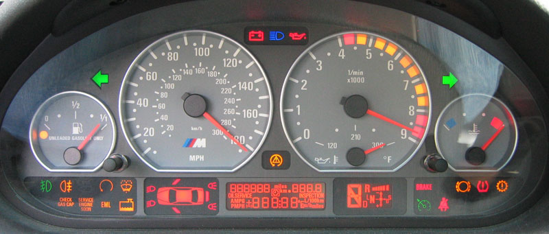
In the newest LCD-based instrument clusters the analogue gauge type displaying will continue to be available as detailed in the following subsection.
4.3.3.2. LCD display
Liquid crystals were first discovered in the late 19th century by the Austrian botanist, Friedrich Reinitzer, and the term liquid crystal itself was coined shortly afterwards by German physicist, Otto Lehmann. The major (from automotive perspective) LCD technologies are shortly detailed in the followings based on [57].
Liquid crystals are almost transparent substances, exhibiting the properties of both solid and liquid matter. Light passing through liquid crystals follows the alignment of the molecules that make them up – a property of solid matter. In the 1960s it was discovered that charging liquid crystals with electricity changed their molecular alignment, and consequently the way light passed through them; a property of liquids.
LCD is described as a transmissive technology because the display works by letting varying amounts of a fixed-intensity white backlight through an active filter. The red, green and blue elements of a pixel are achieved through simple filtering of the white light.
Most liquid crystals are organic compounds consisting of long rod-like molecules which, in their natural state, arrange themselves with their long axes roughly parallel. It is possible to precisely control the alignment of these molecules by flowing the liquid crystal along a finely grooved surface. The alignment of the molecules follows the grooves, so if the grooves are exactly parallel, then the alignment of the molecules also becomes exactly parallel.
In their natural state, LCD molecules are arranged in a loosely ordered fashion with their long axes parallel. However, when they come into contact with a grooved surface in a fixed direction, they line up in parallel along the grooves.
The first principle of an LCD consists of sandwiching liquid crystals between two finely grooved surfaces, where the grooves on one surface are perpendicular (at 90 degrees) to the grooves on the other. If the molecules at one surface are aligned north to south, and the molecules on the other are aligned east to west, then those in-between are forced into a twisted state of 90 degrees. Light follows the alignment of the molecules, and therefore is also twisted through 90 degrees as it passes through the liquid crystals. However, when a voltage is applied to the liquid crystal, the molecules rearrange themselves vertically, allowing light to pass through untwisted.
The second principle of an LCD relies on the properties of polarising filters and light itself. Natural light waves are orientated at random angles. A polarising filter is simply a set of incredibly fine parallel lines. These lines act like a net, blocking all light waves apart from those (coincidentally) orientated parallel to the lines. A second polarising filter with lines arranged perpendicular (at 90 degrees) to the first would therefore totally block this already polarised light. Light would only pass through the second polariser if its lines were exactly parallel with the first, or if the light itself had been twisted to match the second polariser.
A typical twisted nematic (TN) liquid crystal display consists of two polarising filters with their lines arranged perpendicular (at 90 degrees) to each other, which, as described above, would block all light trying to pass through. But in-between these polarisers are the twisted liquid crystals. Therefore light is polarised by the first filter, twisted through 90 degrees by the liquid crystals, finally allowing it to completely pass through the second polarising filter. However, when an electrical voltage is applied across the liquid crystal, the molecules realign vertically, allowing the light to pass through untwisted but to be blocked by the second polariser. Consequently, no voltage equals light passing through, while applied voltage equals no light emerging at the other end.
Basically two LCD control technique exist: passive matrix and active matrix. The earliest laptops (until the mid-1990s) were equipped with monochrome passive-matrix LCDs, later the colour active-matrix became standard on all laptops. Passive-matrix LCDs are still used today for less demanding applications. In particular this technology is used on portable devices where less information content needs to be displayed, lowest power consumption (no backlight) and low cost are desired, and/or readability in direct sunlight is needed.
The most common type of active matrix LCDs (AMLCDs) is the Thin Film Transistor LCD (TFT LCD), which contains, besides the polarizing sheets and cells of liquid crystal, a matrix of thin-film transistors. In a TFT screen a matrix of transistors is connected to the LCD panel – one transistor for each colour (RGB) of each pixel. These transistors drive the pixels, eliminating at a stroke the problems of ghosting and slow response speed that afflict non-TFT LCDs.
The liquid crystal elements of each pixel are arranged so that in their normal state (with no voltage applied) the light coming through the passive filter is polarised so as to pass through the screen. When a voltage is applied across the liquid crystal elements they twist by up to ninety degrees in proportion to the voltage, changing their polarisation and thereby blocking the light’s path. The transistors control the degree of twist and hence the intensity of the red, green and blue elements of each pixel forming the image on the display.
TFT screens can be made much thinner than LCDs, making them lighter, and refresh rates reached the fast 5 ms value.
There are several TFT panel types exist considering the backlight and panel technology.
The LCDs does not produce light itself, thus a proper light source is needed to built-in to produce a visible image. (However low-cost monochrome LCDs are available without backlight.) Until about 2010 the backlight of large LCD panels was based on Cold Cathode Fluorescent Lamps (CCFLs). It has several disadvantages such as higher voltage and power needed, thicker panel design, no high-speed switching, faster aging. The new LED-based backlight technologies eliminated these harmful properties and took over the CCFL.
The panel technologies can be divided into three main groups:
Twisted Nematic (TN)
In Plane Switching (IPS)
VA (Vertical Alignment)
Without going into the technical details of these technologies the main comparable features are given as follows.
The TN panel provides the shortest response time (>1ms), and it is very cost effective technology. On the other hand these panels use only 18 bit colour depth which can be increased virtually, but the colour reproduction is not perfect anyway. Another disadvantage is the poor viewing angle.
The IPS panels’ core strength are the exact colour reproduction and the wide viewing angle. The response time is higher than the TN, but it managed to the proper level (>5ms) by now. Despite the higher costs, all in all the IPS panels is the best TFT LCD panels now.
Considering the properties the VA panels can be located between TN and IPS ones. Considering the contrast ratio it is the best technology, but with higher response time (>8ms) and a medium colour reproduction.
4.3.3.3. OLED display
Today’s cutting-edge display technology is the OLED (organic light emitting diode). It is a flat light emitting technology, made by placing a series of organic (carbon based) thin films between two conductors. When electrical current is applied, a bright light is emitted. OLEDs can be used to make displays and lighting. Because OLEDs emit light, they do not require a backlight and so are thinner and more efficient than LCD displays. OLEDs are not just thin and efficient - they can also be made flexible (even rollable) and transparent.
The basic structure of an OLED is a cathode (which injects electrons), an emissive layer and an anode (which removes electrons). Modern OLED devices use many more layers in order to make them more efficient, but the basic functionality remains the same.
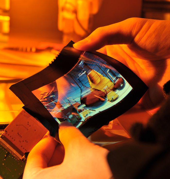
OLED displays have the following advantages over LCD displays:
Lower power consumption
Faster refresh rate and better contrast
Greater brightness and fuller viewing angle
Exciting displays (such as ultra-thin, flexible or transparent displays)
Better durability (OLEDs are very durable and can operate in a broader temperature range)
Lighter weight (the screen can be made very thin)
But OLEDs also have some disadvantages. First of all, today it costs more to produce an OLED than it does to produce an LCD. Although this should hopefully change in the future, as OLEDs has a potential to be even cheaper than LCDs because of their simple design.
OLEDs have limited lifetime (like any display, really), that was quite a problem a few years ago. But there has been constant progress, and today this is almost a non-issue. Today OLEDs last long enough to be used in mobile devices and TVs, but the lifetime of a vehicle is significantly longer. OLEDs can also be problematic in direct sunlight, because of their emissive nature, which also could be a problem in a car. But companies are working to make it better, and newer mobile device displays are quite good in that respect.
Today OLED displays are used mainly in small (2" to 5") displays for mobile devices such as phones, cameras and MP3 players. OLED displays carry a price premium over LCDs, but offer brighter pictures and better power efficiency. Making larger OLEDs is possible, but difficult and expensive now. In 2014 several new OLED TVs has been announced and presented, which shows that the manufacturers are trying to force this promising technology, which will make the lower costs in the future. (Source: [58])
A software configurable instrument cluster is essentially an LCD display behind the steering wheel, which can be customized to different applications (e.g. sport, luxury sedan display or special diagnostic display). There is theme selection with several colour and shape configurations and we can also decide what gauges or windows should appear. Font size altering option could help for the visually impaired. The central console display can also be temporarily ported over to the instrument cluster showing radio channel information or the current image of the parking systems status. The advantage is that the driver does not have to look aside from the instrument panel
Figure 73 shows a BMW instrument panel, which is based on a 10,2”, high-resolution (318 dpi) LED LCD display, with 6:1 aspect ratio.
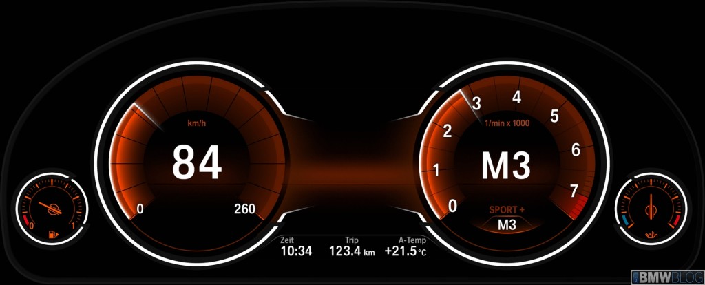
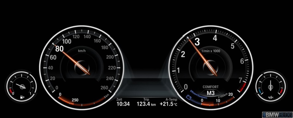
4.3.3.4. Head-Up Display (HUD)
As the name of the display describes the driver can keep his head straight ahead (Head-Up) while looking at displayed information projected onto the windscreen. The driver is able to check e.g. car speed without having to take his eyes off the road. The HUD earlier was used only on cockpits of fighter aircrafts, but today more and more passenger cars took over the technology.
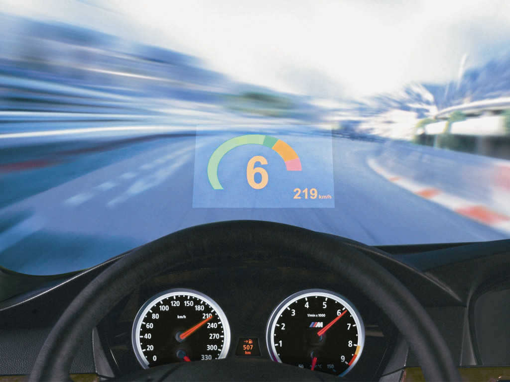
HUD system contains a projector and a system of mirrors that beams an easy-to-read, high-contrast image onto a translucent film on the windscreen, directly in your line of sight. The image is projected in such a way that it appears to be about two metres away, above the tip of the bonnet, making it particularly comfortable to read. BMW claims that Head-Up Display halves the time it takes for eyes to shift focus from road to the instruments and back. The system’s height can be adjusted for optimal viewing. The newest HUDs provides full colour displaying which makes the car even more comfortable for the driver. More colours mean it’s easier to differentiate between general driving information like speed limits and navigation directions and urgent warning signals. Important information like “Pedestrian in the road” is now even more clear and recognisable – and this subsequently reduces the driver’s reaction time. (Source [51])
New technologies like the Head-Up Display (HUD) might be promising solution to reduce the time for the driver to be informed, because the information (road sign, speed limit, hazardous situation) can directly be projected in front of the driver eyes without any distraction. There are researches to use HUD technology on the full windshield that would revolutionize e.g. night vision applications providing road path and obstacle “simulation” feeling to driver (see Figure 75 [59]).
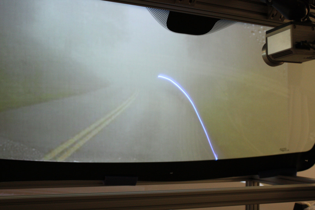
4.3.3.5. Indicator lights (Tell-tales)
Indicator lights are used in the instrument cluster to feedback of the operation of a function or indicate an error. In automotive industry the indicator lights are often called tell-tales. They could be bulbs or LEDs, which lights up a symbol or a text and the colour indicates the priority of the warning. Generally the red colour means an error that requires the car to stop immediately. In case of yellow colour the journey can be continued and it could be investigated later. But in the latter case a safety function may be out of the operation.
Indicator lights are regulated by automobile safety standards worldwide. In the United States, National Highway Traffic Safety Administration Federal Motor Vehicle Safety Standard 101 includes indicator lights in its specifications. In Europe and throughout most of the rest of the world, ECE Regulations specify it, more precisely “United Nations (UN) Vehicle Regulations - 1958 Agreement” [60].
The exact meaning and the usage of other (unregulated) symbols are manufacturer specific in the most cases.
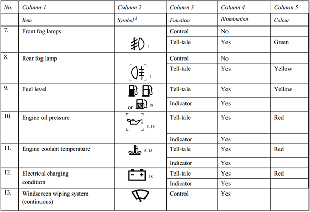
4.3.4. Haptic interfaces
For the haptic channel, haptic feedback components on the steering wheel, the pedals and the driver’s seat are planned. The haptic functions that have already been mentioned in the corresponding sections, can be summarized as follows:
Pedal force and vibration for warning and efficiency functions
Force feedback steering wheel and vibration
Driver’s seat vibration for warning and safety functions
4.4. Driver State Assessment
Driver behaviour monitoring is a special category in the Human-Machine Interface section, since it does not require any direct action from the driver (e.g. pushing, touching, reading, etc.). On the other hand driver state assessment provides very important safety relevant information about the driver’s mental condition, especially drowsiness and attention/distraction which is essential in case of highly automated driving.
The risk of momentarily falling asleep during long-distance driving in the night is quite high. During driver underload situations drivers may easily loose attention, combined with monotony the risk of falling asleep even becomes higher.
Studies show that, after just four hours of non-stop driving, drivers' reaction times can be up to 50 % slower. So the risk of an accident doubles during this time. And the risk increases more than eight-fold after just six hours of non-stop driving! This is the reason why driving time recording devices (tachograph) are mandatory all across Europe for commercial vehicles. (Source: [61])
The driver status is calculated by special algorithms based on direct and indirect monitoring of the driver. The assessment of the driver can be grouped into the following categories:
Drowsiness level
Direct monitoring
Eye movement
Eye blinking time and frequency
Indirect monitoring
Driver activity
Lane keeping
Pedal positions
Steering wheel intensity
Attention/distraction level
Driver look focuses on the street or not
Use of control buttons
Direct driver status monitoring is usually based on a camera (built in the instrument panel or in the inside mirror) that records the driver face, eye movements, blinking time and frequency and determine driver status accordingly.
Indirect monitoring means the evaluation of the driver activity based on other sensor information (e.g. steering wheel movement, buttons/switches). The indirect algorithms calculate an individual behavioural pattern for the driver during the first few minutes of every trip. This pattern is then continuously compared with the current steering behaviour and the current driving situation, courtesy of the vehicle's electronic control unit. This process allows the system to detect typical indicators of drowsiness and warn the driver by emitting an audible signal and flashing up a warning message in the instrument cluster. (Source: [61])
Driver distraction is a leading cause of motor-vehicle crashes. Developing driver warning systems that measure the driver status can help to reduce distraction-related crashes. For such a system, accurately recognizing driver distraction is critical. The challenge of detecting driver distraction is to develop the algorithms suitable to identify different types of distraction. Visual distraction and cognitive distraction are two major types of distraction, which can be described as “eye-off-road” and “mind-offroad”, respectively. (Source: [62])
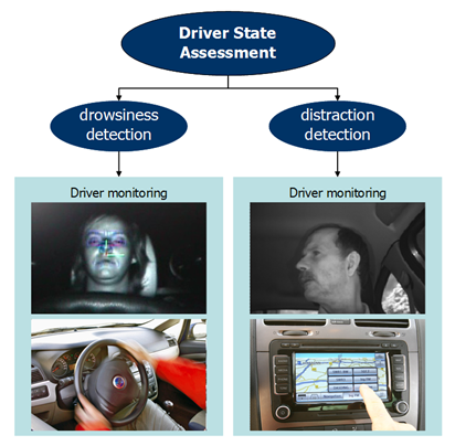
From highly automated driving point of view it is essential to know the status of the driver, whether he is able to take back control in a dangerous situation or a minimum safety risk manoeuvre has to be carried out due to medical emergency of the driver.
Chapter 5. Trajectory planning layer
The potential levels of vehicle automation are determined based on the sensor fusion information of the perception layer. Depending on the availability of the different automation levels the command layer calculates possible vehicle trajectories with priorities ranks of performance and safety. It is the task of the so called auto-pilot to calculate and rank longitudinal or combined longitudinal and lateral trajectory options. At last, taking the driver intention into account the command layer decides the level of automation and selects the trajectory to be executed.
The formulation of the vehicle trajectory, the roadpath that the vehicle travels is composed of two tasks: the trajectory planning and the trajectory execution. Trajectory planning part involves the calculation of different route possibilities with respect to the surrounding environment, contains the ranking, prioritization of the different route options based on minimizing the risk of a collision, and ends up in the selection of the optimum trajectory. The trajectory execution part contains the trajectory segmentation and the generation of the motion vector containing longitudinal and lateral control commands that will be carried out by the intelligent actuators (Section 7) of the execution layer (Section 6).
There are already vehicle automation functions available in series production (e.g. intelligent parking assistance systems) that use trajectory planning and execution. These systems are able to park the car under predefined circumstances without any driver intervention, but there are significant limitations compared to the highly automated driving. The most important difference is that parking assistance systems operate in a static or quasi-static environment around zero velocity, while for example temporary auto-pilot drives the vehicle highly automated around 130 km/h in a continuously and rapidly changing environment.
The output of this layer is a trajectory represented in the motion vector that specifies the vehicle status (position, heading and speed) for the subsequent moments.
5.1. Longitudinal motion
Longitudinal motion control has developed considerably since the beginnings. Started with standard mechanical, later electronic cruise control, passing through the radar extended adaptive cruise control, later including Stop&Go function and arriving at the V2V based cooperative adaptive cruise control system.
Early Cruise Control (CC) functions were only able to maintain a certain engine revolution at the beginning; later systems were capable of holding a predefined speed constantly. This involved longitudinal speed control by using the engine as the only actuator. The extension of the cruise control system with a long range RADAR (Section 3.1) led to the invention of the Adaptive Cruise Control (ACC) system. ACC systems (besides longitudinal speed control) could also keep a speed dependant safe distance behind the ego vehicle. Changing between speed and distance control was automatic based on the traffic situation in front of the vehicle. ACC began to use the brake system as a second actuator. With Stop & Go function, the applicability of ACC was expanded for high-congestion, stop-and-go traffic. ACC with Stop & Go can control longitudinal speed downto zero and back to set speed permitting efficient use in traffic jams. Today’s most advanced ACC systems also take into consideration topographic information from the eHorizon like the curves and slopes ahead to calculate an optimum speed profile for the next few kilometres, see Section 6.1 for details.
In contrast to standard adaptive cruise control (ACC) that uses vehicle mounted radar sensors to detect the distance and the speed of the ego vehicle, Cooperative ACC uses V2V communication for transmitting acceleration data to reduce the time delay of onboard ranging sensors. This enables the following vehicles to adjust their speeds according to the ego vehicle resulting in better distance keeping performance. Figure 78 shows two comparison diagrams for ACC and cooperative ACC, indicating that V2V information exchange instead of external sensor measurement can significantly reduce of the control loop. (Source: [63], [64])
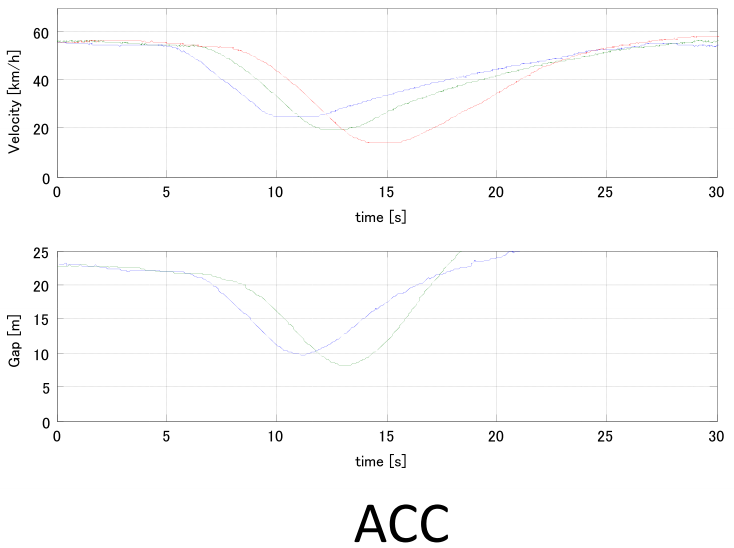
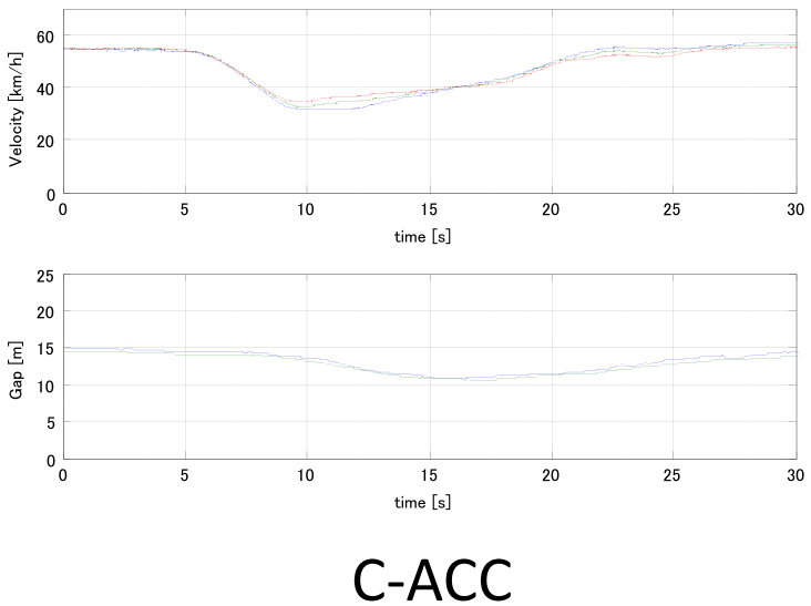
5.2. Lateral motion
Lateral motion control without longitudinal motion control hardly exists, the rare example may be the assisted parking, where the lateral motion control is automated while the longitudinal motion control still remains at the driver.
The objective of assisted parking systems is to improve comfort and safety of driving during parking manoeuvres. Improve comfort by being able to park the vehicle without the driver steering and improve safety by calculating precisely the parking space size and collision-free motion trajectory avoiding any human failures that may occur during a parking manoeuvre. Series production assisted parking systems appeared on the market in the beginning of the 2000s. The advances in electronic technology enabled the development of precise ultrasonic sensors (Section 3.2) for nearby distance measurement and electronic power assisted steering (EPAS, Section 7.3) for driverless steering of the vehicle.
The task of trajectory planning starts with the determination of the proper parking space. By travelling low speed and continuously measuring the vehicle side distance, the parking gap can be calculated, thus proper parking space can be selected. As the first automated parking systems were capable of handling only parallel parking, the initial formulas for trajectory calculation were divided into the following segments:
straight backward path
full (right) steering backward path
straight backward path
full (left) steering backward path
(optional straight forward path)
Depending on the availability of the intelligent actuators in the vehicle the execution of the parking trajectory may also require assisted driver intervention. (Source: [65])
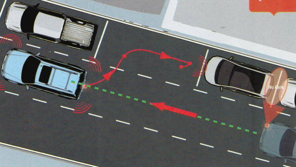
As there are different scenarios exist in everyday parking situations automated parking systems also try to assist the drivers in other situations then just parallel parking. Today’s advanced parking assist systems can also cope with perpendicular or angle parking that require a slightly different approach in lateral motion control.
One topic of recent research in highly automated driving, which is especially challenging in urban environments is fully autonomous parking control. The challenge hereby arises from the narrow corridors, tight turns and unpredictable moving obstacles as well as multiple driving direction switching. The following figure shows common parking spots in urban environments that is subject of the research and development today. (Source: [66])
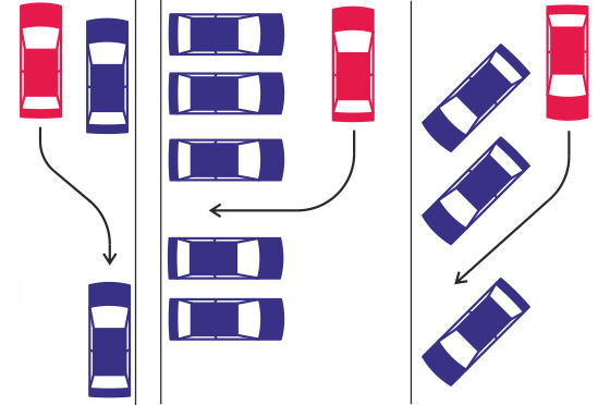
Besides parking another good example of low speed combined longitudinal and lateral control is the traffic jam assist system. At speeds between zero and 40 or 60 km/h (depending on OEMs), the traffic jam assist system keeps pace with the traffic flow and helps to steer the car within certain constraints. It also accelerates and brakes autonomously. The system is based on the functionality of the adaptive cruise control with stop & go, extended by adding the lateral control of steering and lane guidance. The function is based on the built-in radar sensors, a wide-angle video camera and the ultrasonic sensors of the parking system. As drivers spend a great amount of their time in heavy traffic, such systems could reduce the risk of rear-end collisions and protect the drivers mentally by relieving them from stressful driving. (Source: [67])
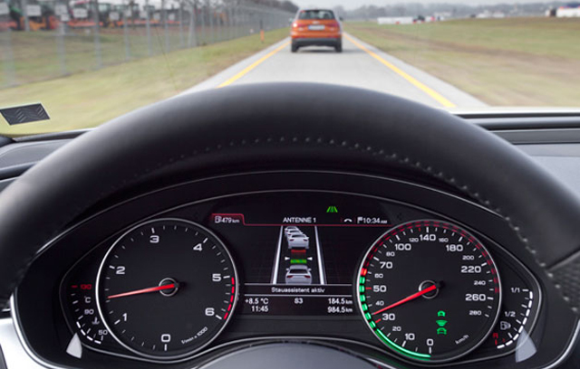
Today’s lane keeping assist (LKA) systems are the initial signs of higher speed lateral control of vehicles. Based on camera and radar information these systems are capable of sensing if the vehicle is deviating from its lane, then they help the vehicle stay inside the lane by an automated steering and/or braking intervention. An advanced extension of LKA is lane centring assist (LCA) when the vehicle not only stays inside the lane but lateral control algorithm keeps the vehicle on a path near the centre of the lane. The primary objective of the lane keeping assist and lane centring assist functions are to warn and assist the driver and these systems are definitely not designed to substitute the driver for steering the vehicle, although on technical level they would be able to do so. (Source: [68], [69])
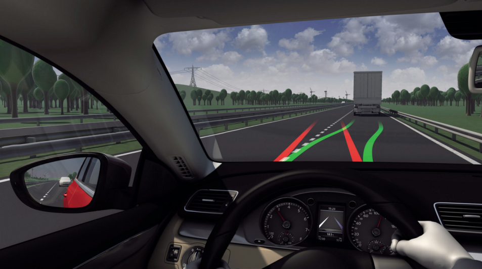
Complex functions like highly automated driving with combined longitudinal and lateral control will definitely appear first on highways, since traffic is more predictable and relatively safe there (one-way traffic only, quality road with relative wide lanes, side protections, good visible lane markings, no pedestrians or cyclists, etc.). As highways are the best places to introduce hands-free driving at higher speeds, one could expect a production vehicle equipped with a temporary autopilot or in other words automated highway driving assist function as soon as the end of this decade.
Automated highway driving means the automated control of the complex driving tasks of highway driving, like driving at a safe speed selected by the driver, changing lanes or overtaking front vehicles depending on the traffic circumstances, automatically reducing speed as necessary or stopping the vehicle in the right most lane in case of an emergency. Japanese Toyota Motor have already demonstrated their advanced highway driving support system prototype in real traffic operation. The two vehicles (shown on Figure 83) communicate each other, keeping their lane and following the preceding vehicle to maintain a safety distance. (Source: [70])
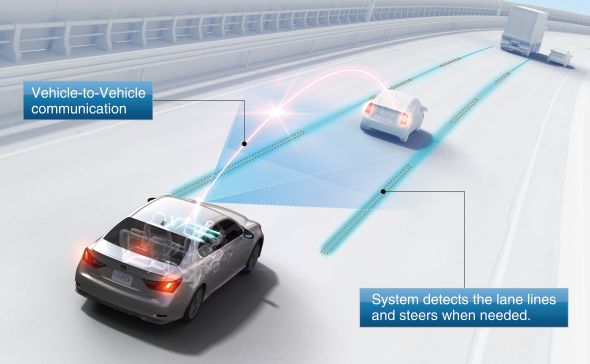
Nissan had also announced that they are also developing their highly automated cars, which is targeted to hit the road by 2020. Equipped with laser scanners, around view monitor cameras, and advanced artificial intelligence and actuators, is not fully autonomous as its systems are designed to allow the driver to manually take over control at any time. As Figure 84 illustrates the highly automated Leaf is being tested in a number of combined longitudinal and lateral control scenarios including automated highway exit, lane change, overtaking vehicles. (Source: [71]
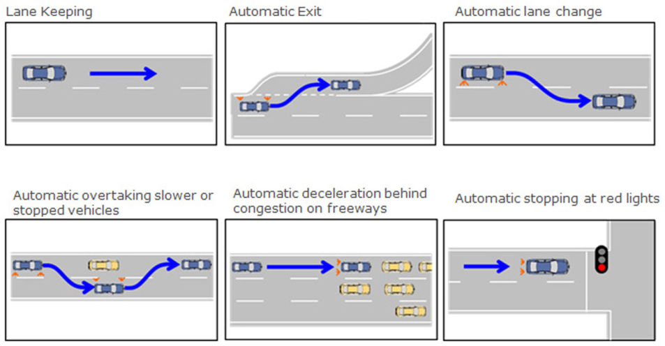
5.3. Automation level
In highly automated vehicles it is always the driver’s decision to pass over control to the vehicle, but to be able to do so certain conditions must be met before. The trajectory planning layer processes vehicle and environment data passed on from the environment sensing (perception) layer as well as the driver's intention, the driver state assessment data and the driver automation level request which is provided by the human machine interface. The driver request for a higher automation can only be fulfilled if the prerequisites are met:
Availability of a higher automation level
Real-time environment sensing
Current status of vehicle dynamics
Driver attention
Driver request for higher automation
The potential automation levels provide only options for the driver requested automation levels. The command layer determines the potential automation levels and enables the system to initiate transitions between different levels based on the driver’s decision.
5.4. Auto-pilot
There is an auto-pilot algorithm responsible for the calculation of potential trajectory and for the selection of the optimum path. The algorithm processes the current situation of the vehicle, the output of the environment sensing (front vehicle, objects, lanes, road, intersection information, etc.) and the intention of the driver (by means of automation level). Finally the auto-pilot system generates the motion vector that will be carried out by the vehicle powertrain controllers and intelligent actuators in order to execute the computed path.
From the results of the multi-sensor based fusion module, the co-pilot algorithms will identify the type of situation the vehicle is in and generate driving strategy options to handle the situation. Driving strategy in this context means a set of feasible manoeuvres and trajectories to be realized by the vehicle or the driver. Driving strategy determination is based upon the analysis of the current driving situation (based on both environment sensor information and future estimation). The assessment of the danger level of the current driving situation may lead the system to select a minimum safety risk strategy or an emergency strategy for the sake of safety. The objective of the auto-pilot is to determine the optimum driving strategy for the driving context.
The co-pilot will provide the set of trajectories with their prioritization. Furthermore, a description of the manoeuvres which the automation intends to perform is provided by these trajectories. Every trajectory is assigned to a specific manoeuvre (e.g. slow down and stop; slow down and steer right; speed up, steer left and overtake) and vice versa. The calculations are based on the input from the perception layer. Irrespective of the automation level, the auto-pilot process is divided into two main functions (Source: [6]):
The definition of a driving strategy at a high level, which is described using a manoeuvre language.
The definition of trajectory at a lower level: this function uses the previously selected manoeuvre to define a reduced possibility field of the trajectory.
The definition of a driving strategy at a high level sub module is based on fast and simple algorithms that evaluate the possibility of several predefined manoeuvres. Some examples of these manoeuvres are “stay in the same lane and accelerate” and “change to the right lane and brake”. Each manoeuvre is ranked by a performance indicator. The aim of this high level is to quickly eliminate a part of the search space, thus reducing the calculation time of the definition of trajectory at low level. It also allows a high level communication towards the driver, in the form of a manoeuvre grid or a manoeuvre tree. There are two ways to represent these manoeuvres: the grid which is a 3x3 matrix, giving 9 cases for the 9 basic manoeuvres plus 1 case for the emergency brake manoeuvre and 1 for the minimum safety risk manoeuvre. Each case is coloured according to its performance indicator (red to orange to yellow to green). The tree representation gives the current situation, and it visualizes the possible actions with their performance indicator as the branches of this tree.
The “definition of trajectory” sub-module describes and evaluates the manoeuvres proposed by the “definition of driving strategy” sub module in greater detail, choosing the best manoeuvres first, until a predefined calculation time span (which is linked to a safe reaction time) elapses.
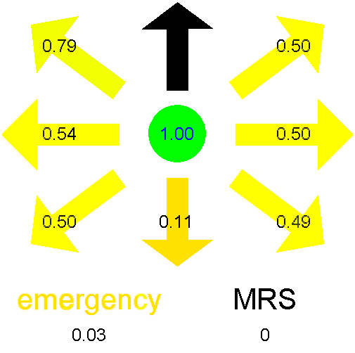
The manoeuvre grid contains the potential longitudinal and lateral actions that the vehicle is capable of performing in its current position. The output of this grid is a ranking of the manoeuvres. The calculation takes into consideration 9 possible combinations that comprise of the multiplication of the 3 longitudinal and 3 lateral options. In the longitudinal direction, the vehicle can accelerate, decelerate (brake) or can keep the current velocity, while in the lateral direction, the vehicle can change lane either to the left or to the right, or can stay in the current lane. There are two additional manoeuvres that have to be considered during the potential manoeuvre calculation, the minimum safety risk manoeuvre and the emergency manoeuvre with maximum braking till standstill. This gives a total of eleven manoeuvres. Each manoeuvre gets a performance indication number between zero and one.
When there are several potential vehicle trajectories available that do not contain the risk of a collision, then the next task is a more detailed evaluation to select the optimum trajectory from them. For being able to select the optimum path, the potential trajectories are ranked and optimized through qualitative and quantitative evaluation according to key performance indicators like:
trajectory complexity
travelling time
driving comfort
fuel consumption
safety margins
The manoeuvre grid algorithm attributes a performance to each of the presented manoeuvres. This is done through the evaluation of a set of performance indicators that are linked with the aspects of good driving. The algorithm measures the risk of collisions with other objects if the manoeuvre would be executed. The total performance of each manoeuvre is the weighted sum of the different performance indicators. Manoeuvres that correspond to a fast and smooth drive without risk or offence against the traffic rules are promoted in the ranking of the manoeuvre grid. The overall weighted performance indicator is presented above; it is used by the manoeuvre fusion algorithm.
According to the assumed driving situation on Figure 86, the best manoeuvre - taking into consideration the trajectory ratings of the grid and tree performance indicators- is overtaking and acceleration in the left lane.
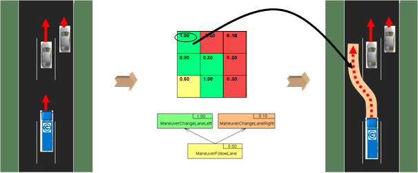
5.5. Motion vector generation
At the end of the trajectory planning the motion control vector is generated based on the output of the environment sensing layer, the auto-pilot and the automation mode selector. The motion control vector contains the desired longitudinal and lateral control demands (and constraints) to be executed by the vehicle. As an interface vector it is passed on to the execution layer and will be executed by the powertrain controllers and the intelligent actuators.
Chapter 6. Trajectory execution layer
The algorithms presented in the previous section compute the vehicle actions to be carried out in order to achieve the required automation task according to all inputs (automation level, driver automation level request, set of trajectories, relevant detected targets, vehicle positioning, trajectory & state limits, vehicle state). The outputs of this function are primarily the trajectory and the speed constraints. This trajectory has to be realized by a control system considering the fuel economy, the speed constraints and vehicle parameters.
Another task of the trajectory execution layer is the execution of the calculated control commands (motion vector) and to provide feedback about the actual status. The motion vector contains the selected trajectory that has to be followed including the desired longitudinal and lateral movement of the vehicle.
The execution of the motion vector is distributed among the intelligent actuators of the vehicle. The task distribution and the harmonization of the intelligent actuators are carried out by the integrated vehicle (powertrain) controller.
6.1. Longitudinal control
The main task of the longitudinal control is the calculation and execution of an optimal speed profile. It is basically a speed control (cruise control) which tries to hold speed set-point given by the driver, but it could be extended by distance control (ACC) and the road inclinations in front of the vehicle. This control method and the extension to a platoon is detailed in the following subsections.
6.1.1. Design of speed profile
The purpose is to design speed trajectory, with which the longitudinal energy, thus fuel requirement can be reduced. If the inclination of the road and the speed limits are assumed to be known, the speed trajectory can be designed. By choosing the speed fitting in these factors the number of unnecessary accelerations and brakes can be reduced.
The road ahead of the vehicle is divided into several sections and reference speeds are selected for them, see Figure 87. The rates of the inclinations of the road and those of the speed limits are assumed to be known at the endpoints of each section. The knowledge of the road slopes is a necessary assumption for the calculation of the velocity signal. In practice the slope can be obtained in two ways: either a contour map which contains the level lines is used, or an estimation method is applied. In the former case a map used in other navigation tasks can be extended with slope information. Several methods have been proposed for slope estimation. They use cameras, laser/inertial profilometers, differential GPS or a GPS/INS systems, see [72], [73], [74]. An estimation method based on a vehicle model and Kalman filters was proposed by [75].
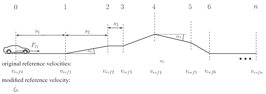
The simplified model of the longitudinal dynamics of the vehicle is shown in Figure 88. The longitudinal movement of the vehicle is influenced by the traction force  as the control signal and disturbances
  . Several longitudinal disturbances influence the movement of the vehicle. The rolling resistance is modeled by an empiric form
  where
where  is the vertical load of the wheel,
  and
and  are empirical parameters depending on tyre and road conditions and
  is the velocity of the vehicle, see GOTOBUTTON GrindEQbibitem24 . The aerodynamic force is formulated as
  where
where  is the drag coefficient,
  is the density of air,
  is the reference area,
  is the velocity of vehicle relative to the air. In case of a lull
  , which is assumed in the paper. The longitudinal component of the weighting force is
  , where m is the mass of the vehicle and
  is the angle of the slope. The acceleration of the vehicle is the following:
  , where
  is the mass of the vehicle,
  is the position of the vehicle, and
  are the traction force and the disturbance force (
 ), respectively.
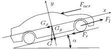
Although between the points may be acceleration and declaration an average speed is used. Thus, the rate of accelerations of the vehicle is considered to be constant between these points. In this case the movement of the vehicle using simple kinematic equations is:  , where
  is the velocity of vehicle at the initial point,
  is the velocity of vehicle at the first point and
  is the distance between these points. Thus the velocity of the first section point is the following:
  . The velocity of the first section point
  is defined as the reference velocity
  . This relationship also applies to the next road section:
  . It is important to emphasize that the longitudinal force
  is known only the first section. Moreover, the longitudinal forces
  are not known during the traveling in the first section. Therefore at the calculation of the control force it is assumed that additional longitudinal forces will not act on the vehicle, i.e., the longitudinal forces
  will not affect the next sections. At the same time the disturbances from road slope are known ahead. Similarly, the velocity of the vehicle can be formalized in the next
  section points. Using this principle a velocity-chain, which contains the required velocities along the way of the vehicle, is constructed. At the calculation of the control force it is assumed that additional longitudinal forces
  will not affect the next sections. The velocities of vehicle are described at each section point of the road by using similar expressions to GOTOBUTTON GrindEQequation22 . The velocity of the
  section point is the following:
  . It is also an important goal to track the momentary value of the velocity. It can also be considered in the following equation:
The  disturbance force can be divided in two parts: the first part is the force resistance from road slope
  , while the second part
  contains all of the other resistances such as rolling resistance, aerodynamic forces etc. We assume that
  is known while
  is unknown.
  depends on the mass of the vehicle and the angle of the slope
  . When the control force
  is calculated, only
  influences the vehicle of all of the unmeasured disturbances. In the control design the effects of the unmeasured disturbances
  are ignored. The consequence of this assumption is that the model does not contain all the information about the road disturbances, therefore it is necessary to design a robust speed controller. This controller can ignore the undesirable effects. Consequently, the equations of the vehicle at the section points are calculated in the following way:
| (1) |

| (2) |
| (3) |

| (4) |
The vehicle travels in traffic and it may happen that the vehicle is overtaken. Because of the risk of collision it is necessary to consider the preceding velocity on the lane:
| (5) |

The number of the segments is important. For example in the case of flat roads it is enough to use relatively few section points because the slopes of the sections do not change abruptly. In the case of undulating roads it is necessary to use relatively large number of section points and shorter sections, because it is assumed in the algorithm that the acceleration of the vehicle is constant between the section points. Thus, the road ahead of the vehicle is divided unevenly, which is consistent with the topography of the road.
In the following step weights  are applied to reference speeds. An additional weight
  is applied to the momentary speed. An additional weight
  is applied to the leader speed. While the weights
  represent the rate of the road conditions, weight
  has an essential role: it determines the tracking requirement of the current reference velocity
  . By increasing
  the momentary velocity becomes more important while road conditions become less important. Similarly, by increasing
  the road conditions and the momentary velocity become negligible. The weights should sum up to one, i.e.
  .
.
Weights have an important role in control design. By making an appropriate selection of the weights the importance of the road condition is taken into consideration. For example when  and
and  the control exercise is simplified to a cruise control problem without any road conditions. When equivalent weights are used the road conditions are considered with the same importance, i.e.,
  and
and  . When
  and
and  only the tracking of the preceding vehicle is carried out. The optimal determination of the weights has an important role, i.e., to achieve a balance between the current velocity and the effect of the road slope. Consequently, a balance between the velocity and the economy parameters of the vehicle is formalized.
By summarizing the above equations the following formula is yielded:
| (6) |
where the value  depends on the road slopes, the reference velocities and the weights
| (7) |
In the final step a control-oriented vehicle model, in which reference velocities and weights are taken into consideration, is constructed. The momentary acceleration of the vehicle is expressed in the following way:  where
where  . Equation (6) is rearranged:
| (8) |

where the parameter  is calculated based on the designed
  . Consequently, the road conditions can be considered by speed tracking. The momentary velocity of vehicle
  should be equal to parameter
  , which contains the road information. The calculation of
  requires the measurement of the longitudinal acceleration
  .
.
6.1.2. Optimization of the vehicle cruise control
In the following step the task is to find an optimal selection of the weights in such a way that both the minimization of control force and the traveling time are taken into consideration. Equation (6) shows that  depends only on the weights in the following way:
| (9) |

Since  depends on the weight
  , therefore
  depends on the weights
  and
and  . The longitudinal control force must be minimized, i.e.,
  . Instead, in practice the
  optimization is used because of the simpler numerical computation. Simultaneously, the difference between momentary velocity and modified velocity must be minimized, i.e.,
The two optimization criteria lead to different optimal solutions. In the first criterion the road inclinations and speed limits are taken into consideration by using appropriately chosen weights  . At the same time the second criterion is optimal if the information is ignored. In the latter case the weights are noted by
  . The first criterion is met by the transformation of the quadratic form into the linear programming using the simplex algorithm. It leads to the following form:
  with the following constrains
  and
and  . This task is nonlinear because of the weights. The optimization task is solved by a linear programming method, such as the simplex algorithm.
The second criterion must also be taken into consideration. The optimal solution can be determined in a relatively easy way since the vehicle tracks the predefined velocity if the road conditions are not considered. Consequently, the optimal solution is achieved by selecting the weights in the following way:  and
and  .
.
In the proposed method two further performance weights, i.e.,  and
and  , are introduced. The performance weight
  (
( ) is related to the importance of the minimization of the longitudinal control force
  while the performance weight
  is related to the minimization of
  . There is a constraint according to the performance weights
  . Thus the performance weights, which guarantee balance between optimizations tasks, are calculated in the following expressions:
| (10) |
 , i=1,n(11)
Based on the calculated performance weights the speed can be predicted.
The tracking of the preceding vehicle is necessary to avoid a collision, therefore  is not reduced. If the preceding vehicle accelerates, the tracking vehicle must accelerate as well. As the velocity increases so does the braking distance, therefore the following vehicle strictly tracks the velocity of the preceding vehicle. On the other hand it is necessary to prevent the velocity of the vehicle from increasing above the official speed limit. Therefore the tracked velocity of the preceding vehicle is limited by the maximum speed. If the preceding vehicle accelerates and exceeds the speed limit the following vehicle may fall behind.
Remark 3.1 Look-ahead control considering efficiency and safe cornering
The maximum cornering velocity for each section can be calculated in advance knowing the designed path of the vehicle. If the speed limit  at section point
  exceeds the safe cornering velocity then the speed limit
  is substituted with the smallest value concerning skidding or rollover, i.e.,
| (12) |

6.1.3. Implementation of the velocity design
The control system can be realized in three steps as Figure 89 shows. The aim of the first step is the computation of the reference velocity. The results of this computation are the weights and the modified velocity which must be tracked by the vehicle. In the second step the longitudinal control force of the vehicle ( ) is designed. The role of the high-level controller is to calculate this required longitudinal force. In third step the real physical inputs of the system, such as the throttle, the gear position and the brake pressure are generated by the low-level controller.
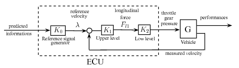
In the proposed method the steps are separated from each other. The reference velocity signal generator can be added to the upper-lower Adaptive Cruise Control (ACC) system. It is possible to design a reference signal generator unit almost individually, and to attach it to the ACC system. Thus the reference signal unit can be designed and produced independently from automobile suppliers, only a few vehicle data are needed. The independent implementation possibility is an important advantage in practice. The high-level controller calculates positive and negative forces as well, therefore the driving and braking systems are also actuated. Figure 90 shows the architecture of the low-level controller.
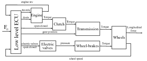
The engine is controlled by the throttle, which could be a butterfly gate or a quantity of injected fuel. The engine-management system and the fuel-injection system have their own controllers, thus in the realization of the low-level controller only the torque-rev-load characteristics of the engine are necessary. In this case the rev of the engine is measured, the required torque is computed from the longitudinal force of the high-level controller, thus the throttle is determined by an interpolation step using a look-up table. The position of the automatic transmission is determined by logic functions, thus it depends on the fuel consumption and the maximum rev of the engine. The pressures on the cylinders of the wheels increase during braking. At normal traveling the ABS actuation is not necessary, in case of an emergency the optimal driving is overwritten by the safety requirements. The necessary braking pressure for the required braking force is computed from the ratios of the hydraulic/pneumatic parts.
In the simulation example a transportational route with real data is analyzed. The terrain characteristics and geographical information are those of the M1 Hungarian highway between Tatabánya and Budapest in a  -
- -long section. In the simulation a typical F-Class truck travels along the
  route. The mass of the 6--gear truck is
  and its engine power is
  (
( ). The regulated maximal velocity is
  , but the road section contains other speed limits (e.g.
  or
or  ), and the road section also contains hilly parts. Thus, it is an acceptable route for the analysis of road conditions, i.e., inclinations and speed limits. Publicly accessible up-to-date geographical/navigational databases and visualisation programs, such as Google Earth and Google Maps, are used for the experiment.
|
|
|
|
|
|
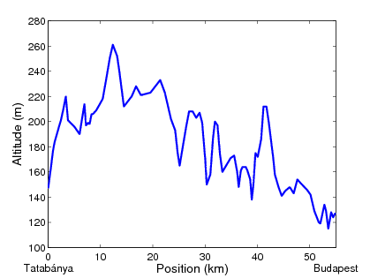
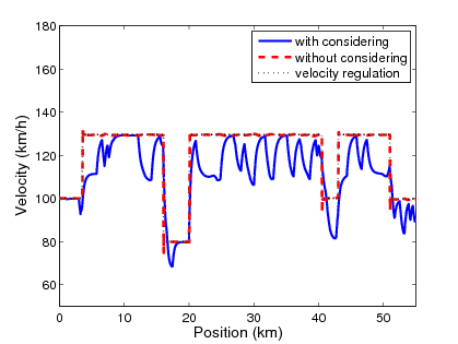
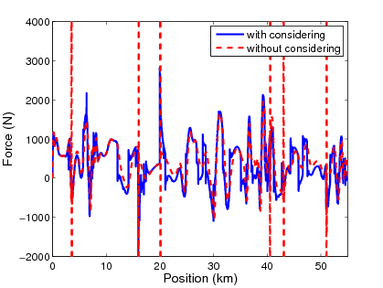
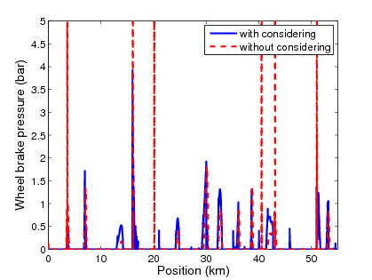
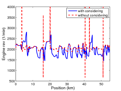
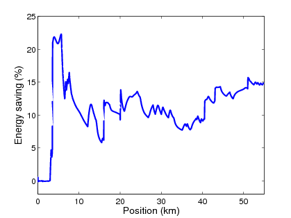
Figure 91: Real data motorway simulation
In this example two different controllers are compared. The first is the proposed controller, which considers the road conditions such as inclinations and speed limits and is illustrated by solid line in the figures, while the second controller is a conventional ACC system, which ignores this information and is illustrated by dashed line. Figure 91 shows the time responses of the simulation.
Figure 91(a) shows that the motorway contains several uphill and downhill sections. Figure 91(b) shows the velocity of the vehicle with speed limits in both cases. The conventional ACC system tracks the predefined speed limits as accurately as possible and the tracking error is minimal. In the proposed method the speed is determined by the speed limits and simultaneously it takes the road inclinations into consideration according to the optimal requirement. Figure 91(c) shows the required longitudinal force. The high-precision tracking of the predefined velocities in the conventional ACC system often requires extremely high forces with abrupt changes in the signals. As a result of the road conditions less energy is required during the journey in the proposed control method, see Figure 91(f). The proposed method requires smaller energy ( ) than the conventional method (
 ), and the energy saving is
  , which is
  . The fuel consumption can also be calculated by using the following approximation:
  where
where  is the efficiency of the driveline system,
  is the heat of combustion and
  is the density of petrol. The fuel consumption of the conventional system is
  while that of the proposed method is
  , which results in
  reduction in fuel consumption in the analyzed
  length section.
Remark 3.2 Speed control based on the preceding vehicle
In addition to the consideration of road conditions it is also important to consider the traffic environment. It means that the preceding vehicle must be considered in the reference speed design because of the risk of collision. Thus, all of the kinetic energy of the vehicle is dissipated by friction. This estimation of the safe stopping distance may be conservative in a normal traffic situation, where the preceding vehicle also brakes, therefore the distance between the vehicles may be reduced. In this paper the safe stopping distance between the vehicles is determined according to the 91/422/EEC, 71/320/EEC UN and EU directives (in case of  vehicle category, the velocity in
  ):
):  . It is also necessary to consider that without the preceding vehicle the consideration of safe stopping distance is neither possible nor necessary. The consideration of the preceding vehicle is determined by
  . The following example analyses the incidence when another vehicle overtakes the vehicle with an adaptive control proposed in the paper or the vehicle catches up with a preceding vehicle.
In the simulation example, the preceding vehicle is slower, however, in the second part its velocity is higher than that of the follower vehicle. Furthermore, in the example the preceding vehicle also exceeds the official speed limit ( ). Figure 92(a) and Figure 92(b) show that in the first part of the simulation the follower vehicle approaches the preceding vehicle taking the braking distance into consideration, while in the second part the follower vehicle avoids exceeding the speed limit and falls behind. This velocity control is achieved by using the value of
  as it is shown in Figure 92(d). In the first part of the simulation the weight is increased by the risk incident while in the second part it is reduced by the increasing distance. The solution requires radar information, which is available in a conventional adaptive cruise control vehicle. This simulation example shows that the designed control system is able adapt to external circumstances.
|
|
|
|
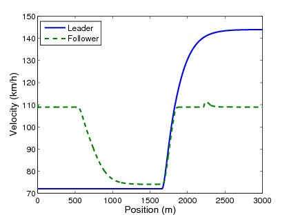
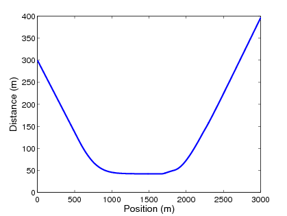
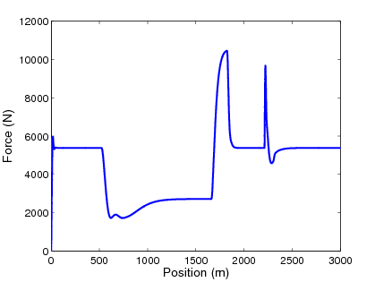
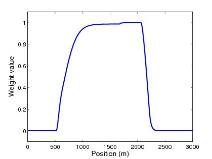
Figure 92: Adaptive control systems with a preceding vehicle
6.1.4. Extension of the method to a platoon
The main idea behind the design is that each vehicle in the platoon is able to calculate its speed independently of the other vehicles. Since traveling in a platoon requires the same speed, the optimal speed must be modified according to the other vehicles. In the platoon, the speed of the leader vehicle determines the speed of all the vehicles. The goal is to determine the common speed at which the speeds of the members are as close as possible to their own optimal speed. In the case of a platoon each vehicle has its own optimal reference speed  . Moreover, speeds of the vehicles are not independent of each other, because the speed of the leader
  influences the speed of every member of platoon
  . The goal is to find an optimal reference speed for the leader
  .
.
It is important to note that there is an interaction between the speeds of the vehicles in a platoon. If a preceding vehicle changes its speed, the follower vehicles will modify their speeds and track the motion of the preceding vehicle within a short time. The members of the platoon are not independent of the leader, therefore it is necessary to formulate the relationship between the speed of the  platoon member
  and the leader and the preceding vehicles. It is formulated with a transfer function with its input and output. The output
  contains the information, i.e., the position, speed and acceleration of the vehicle, which is sent to the follower vehicles. The input
  contains the position, speed, the acceleration of the preceding vehicle and the leader. The transfer function between
  and
and  is
is  with the controller of the
  vehicle
  and its longitudinal dynamics
  . Similarly, the effect of the leader and the preceding vehicles on the
  platoon member is formulated:
  , where
  , which finally leads to
  . Consequently, the speed of the
  vehicle is determined by the next formula:
  . The value of
  is used for the computation of the optimal reference speed of the platoon
  .
.
Finally the required reference speed of the leader vehicle  is designed. The aim of the design is that the generated speeds of all the vehicles
  are as close to as their modified reference speed
  as possible:
| (13) |
Since the speed of the  vehicle is formulated as
  , the following optimization form is used:
  , where
  . It can be stated that in GOTOBUTTON GrindEQequation48 the only unknown variable is
  . The optimization leads to the following equation:
  The solution of the optimization problem can be achieved. The deduction of the optimization of
  is as follows:
| (14) |
It means that the leader vehicle must track the required reference speed  .
.
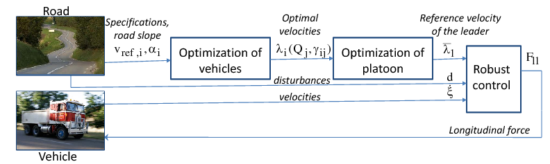
6.2. Lateral control
6.2.1. Design of trajectory
Government transportation agencies have been evaluating several studies in the field of highway road planning in respect to horizontal curve design. Road design manuals determine a minimum curve radius for a predefined velocity, road superelevation and adhesion coefficient, see [76], [77]. The calculation is based on assuming the vehicle to move on a circular path, where the vehicle is subject to centrifugal force that acts away from the center of the curve as illustrated in Figure 94, see [78]. The slip angle  is assumed to be small enough for the lateral force to point along the path radius, and the longitudinal acceleration is also small enough not to degrade the lateral friction of the vehicle considerably.
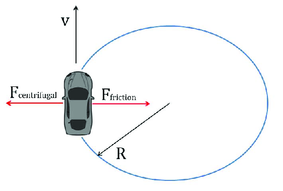
The mass of the vehicle  along with the road superelevation (cross slope)
  and the side friction between the tire and the road surface
  counterbalance the centrifugal force. Assuming that there is the same
  at each wheel of the vehicle the sum of the lateral forces is:
  , where
  is the gravitational constant. At cornering the dynamics of vehicle is described by the equilibrium of the two forces:
  , where
  is the radius of the curve. Assuming that the road geometry is known by on-board devices such as GPS, it is possible to calculate a safe cornering velocity.
The following relationship holds for the maximum safe cornering velocity regarding the danger of skidding out of the corner:
| (15) |
(15) is also used in crash reconstruction and is referred to as the Critical Speed Formula (CSF), see [79], [80]. In the so-called yaw mark method the critical speed of the vehicle is determined by using the calculated radius of the vehicle path from the tire skid marks left on the road.
Note that in the calculation of the safe cornering velocity the value of the side friction factor  plays a major role. This factor depends on the quality and the texture of the road, the weather conditions and the velocity of the vehicle and several other factors. The estimation of
  has been presented by several important papers, see e.g. [81], [82], [83]. However, these estimations are based on instant measurements, thus they are not valid for look-ahead control design, where the friction of future road sections should be estimated.
In road design handbooks the value of the friction factor is given in look-up tables as a function of the design speed, and it is limited in order to determine a comfortable side friction for the passengers of the vehicle. For the calculation of safe cornering velocity these friction values give a very conservative result.
A method to evaluate side friction in horizontal curves using supply-demand concepts has been presented by [84]. Here the side friction has an exponential relation with the design speed as follows:
| (16) |
where  and
and  are constant values depending on the texture of the pavement. Note that
  is the estimated reference friction at a measurement speed of
  . Thus, by using (15) and (16) the maximum safe cornering speed can be determined on a given road surface along with the side friction factor, as it is illustrated inFigure 95. The intersections of the supply and demand curves give the safe cornering velocities and the corresponding maximum side frictions. Note that whereas the friction supply only depends on the velocity of the vehicle, the friction demand is a function of the velocity and the curve radius as well.
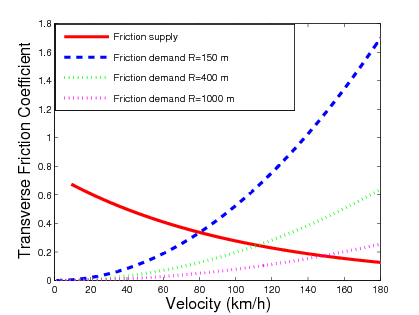
The relationship between the curve radius and safe cornering velocity can be observed in Figure 5. The data points of the diagram are given by the intersections of the supply and demand curves. It shows that the safe cornering velocity increases with the curve radius. However, the relationship is not linear, i.e by increasing an already big cornering radius results in only moderated growth of the safe cornering velocity.
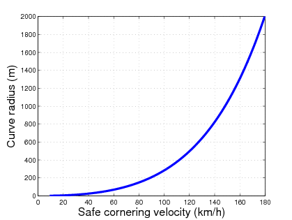
Rollover danger estimation and prevention control methods have already been studied by several authors, see [85], [86], [87]. A quasi-static analysis of maximal safe cornering velocity regarding the danger of rollover has been presented by [88]. Assuming a rigid vehicle and using small angle approximation for superelevation ( ,
,  ), a moment equation can be written for the outside tires of the vehicle during cornering as follows:
| (17) |
where  is the height of the center of gravity,
  is the track width,
  is the load of the inside wheel at cornering.
The vehicle stability limit occurs at the point when the load  reaches zero, which means the vehicle can no longer maintain equilibrium in the roll plane. Thus by reorganizing (17) and substituting
  the rollover threshold is given as follows:
| (18) |
Thus, to ensure safe cornering of the vehicle in a cornering maneuver without the danger of skidding or rollover, the velocity of the vehicle has to chosen to meet the two constraints defined by (15) and (16).
6.2.2. Road curve radius calculation
Another important task is to calculate the radius of curves ahead of the vehicle in order to define the safe cornering velocities in advance. The road ahead of the vehicle can be divided into  number of sections. The goal is to calculate the curve radius at each
  section points ahead of the vehicle to determine the safe cornering velocities corresponding to the curve radius.
The calculation of the cornering radius  ,
,  is as follows. It is assumed that the global trajectory coordinates
  and
and  of the vehicle path are known. Considering a sufficiently small distance the trajectory of the vehicle around a section point can be regarded as an arc, as it is shown in Figure 97. The arc can be divided into
  data points.
The length of the arc can be approximated by summing up the distances between data points:  These distances are calculated as:
  The length of the chord
  is calculated as follows:
  Knowing the length
  and
and  ,
,  it is possible to calculate a reasonable estimation of the curve radius
  . Note that the length of the arc must be chosen carefully. A too short section with fewer data points may give an unacceptable approximation of the radius. On the other hand a too big distance can be inappropriate as well, since then the section may not be approximated by a single arc. The number of data points selected is also important, and by increasing the number
  , the accuracy of the following calculation can be enhanced. The angle of the arc
  is as follows
  . The length of the chord
  is also expressed as a function of the radius:
  . Expressing the radius
  the following equation is derived:
| (19) |
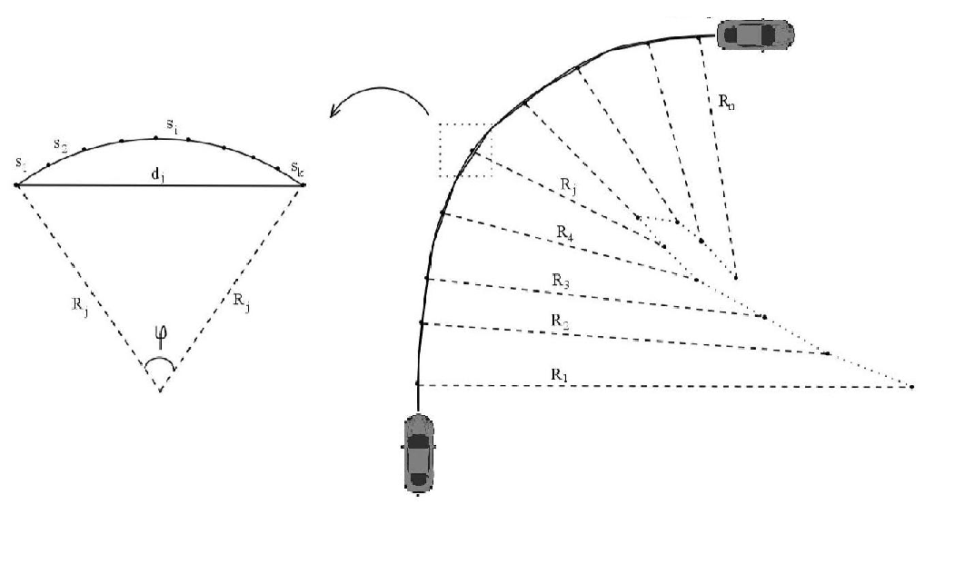
This expression can be transformed by introducing  and using the Taylor series for the approximation of the
  function, i.e.,
  . Then the following expression is gained for the radius:
| (20) |
The curve radius  ,
,  can be calculated at each section point ahead of the vehicle path. The calculation method is validated through the CarSim simulation environment. Here, the vehicle follows the desired path while the curve radius is being measured and at the same time the calculation method is running giving a close approximation of the real value. The comparison of the real and the calculated radius is shown in Figure 98.
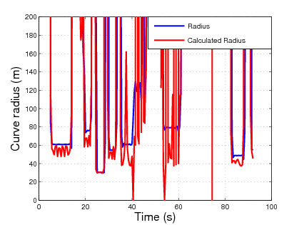
By calculating the radius of the curve using (20) the safe cornering velocity of the vehicle can be determined by using (15) and (18). This velocity can be considered as the maximum velocity that the vehicle is capable of in a corner without the danger of slipping and leaving the track or rolling over. It is important to state that in severe weather conditions this safe velocity may be smaller than that of the speed limit, thus the consideration of the maximum safety velocity in the cruise control design is essential.
Chapter 7. Intelligent actuators
In highly automated driving mode the previously calculated and selected trajectory should be followed by the vehicle. The trajectory path is executed by an intelligent system that has the command vector as an input and drive-by-wire actuators on the output. The trajectory execution layer is composed of drive-by-wire (x-by-wire) subsystems like
Throttle-by-wire
Steer-by-wire
Brake-by-wire
Shift-by-wire
Drive-by-wire systems control the specific vehicle subsystem without mechanical connections, just through electronic (wire) control. The technology has a longer history in the aerospace industry, introducing the first full by-wire controlled aircraft, the Airbus A320 in 1987.
Up until the late 1980s most of the cars have had mechanical, hydraulic or pneumatic connection (such as throttle Bowden cable, steering column, hydraulic brake etc.) between the HMI and the actuator. Series production of the x-by-wire systems was introduced with the throttle-by-wire (electronic throttle control) applications in engine management, where the former mechanical Bowden was replaced for electronically controlled components. The electronic throttle control (ETC) was the first so called x-by-wire system, which has replaced the mechanical connection. The use of ETC systems has become a standard on vehicle systems to allow advanced powertrain control, meet and improve emissions, and improve driveability. Today throttle-by-wire applications are standard in all modern vehicle models. (Source: [89])
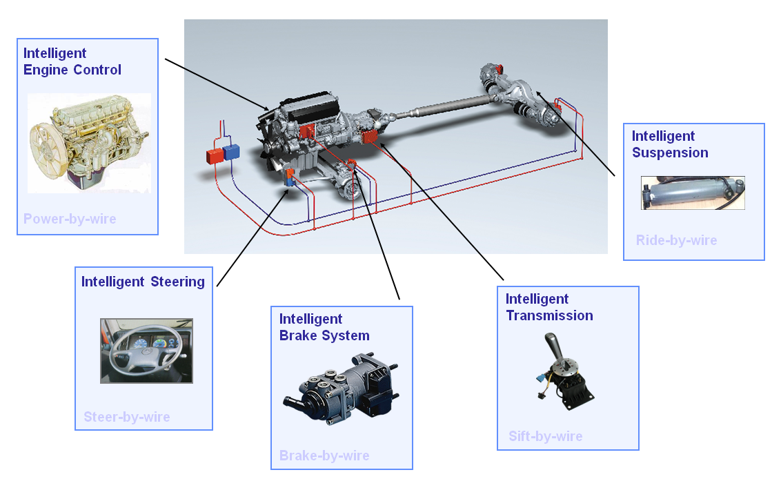
The figure above shows the intelligent actuators in the vehicle that has strong influence on the vehicle dynamics. Throttle–by-wire systems enables the control of the engine torque without touching the gas pedal, steer-by-wire systems allow autonomous steering of the vehicle, brake-by-wire systems delivers distributed brake force without touching the brake pedal, shift-by-wire systems enables the automatic selection of the proper gear.
For providing highly automated vehicle functions the intelligent actuators are mandatory requirements. For example for a basic cruise control function, only the throttle-by-wire actuator is required, but if we extend the functionality for adaptive cruise control the brake-by-wire subsystem will also be a prerequisite. While adding the shift-by-wire actuator one can provide even more comfortable ACC function. Steer-by-wire subsystems become important when not only the longitudinal, but also the lateral control of the vehicle is implemented e.g. lane keeping, temporary autopilot.
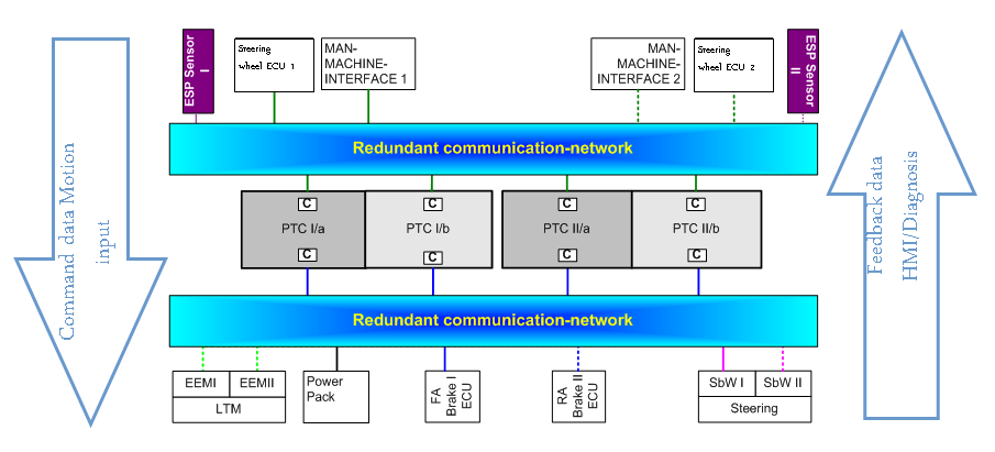
These intelligent actuators are each responsible for a particular domain of the vehicle dynamics control, while the whole vehicle movement (trajectory execution) is organized by the so-called powertrain controller. The powertrain controller separates and distributes the complex tasks for fulfilling the vehicle movement defined by the motion vector.
Another system should be noted here, namely the active suspension system. The suspension is not a typical actuator because generally it is a springing-damping system which connects the vehicle to its wheels, and allows relative movement between each other. The driver cannot influence the movement of the vehicle by direct intervention into the suspension. Modern vehicles can provide active suspension system primarily to increase the ride comfort and additionally to increase vehicle stability, thus safety. In this case an electronic controller can influence the vehicle dynamics by the suspension system.
7.1. Vehicular networks
In automotive industry several communication networks are used parallel, see [90]. In this subsection the CAN technology is detailed because it is the most widespread standard in the field of powertrain applications.
The Controller Area Network (CAN) is a serial communications protocol which efficiently supports distributed real-time control with a very high level of security. Its domain of application ranges from high-speed networks to low-cost multiplex wiring. In automotive electronics, electronic control units (ECU) are connected together using CAN and changing information with each-other by bitrates up to 1 Mbit/s.
CAN is a multi-master bus with an open, linear structure with one logic bus line and equal nodes. The number of nodes is not limited by the protocol. Physically the bus line (Figure 6) is a twisted pair cable terminated by termination network A and termination network B. The locating of the termination within a CAN node should be avoided because the bus lines lose termination if this CAN node is disconnected from the bus line. The bus is in the recessive state if the bus drivers of all CAN nodes are switched off. In this case the mean bus voltage is generated by the termination and by the high internal resistance of each CAN nodes receiving circuitry. A dominant bit is sent to the bus if the bus drivers of at least one unit are switched on. This induces a current flow through the termination resistors and, consequently, a differential voltage between the two wires of the bus. The dominant and recessive states are detected by transforming the differential voltages of the bus into the corresponding recessive and dominant voltage levels at the comparator input of the receiving circuitry.
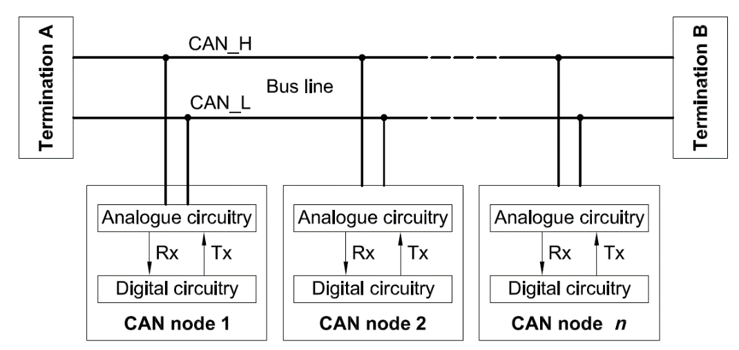
The CAN standard (see [91], [92]) gives specification which will be fulfilled by the cables chosen for the CAN bus. The aim of these specifications is to standardize the electrical characteristics and not to specify mechanical and material parameters of the cable. Furthermore the termination resistor used in termination A and termination B will comply with the limits specified in the standard also.
Besides the physical layer the CAN standard also specifies the ISO/OSI data link layer as well. CAN uses a very efficient media access method based on the arbitration principle called "Carrier Sense Multiple Access with Arbitration on Message Priority". Summarizing the properties of the CAN network the CAN specifications are as follows:
prioritization of messages
event based operation
configuration flexibility
multicast reception with time synchronization
system wide data consistency
multi-master
error detection and signalling
automatic retransmission of corrupted messages as soon as the bus is idle again
distinction between temporary errors and permanent failures of nodes and autonomous switching off of defect nodes
These properties enable the CAN technology to use in automotive environment and especially in safety critical systems. Although the limitations of CAN recently induced the development of new bus systems like FlexRay with higher bandwidth, deterministic time-triggered operation and fault-tolerant architecture, CAN still will be inevitable in the automotive industry for the next decade.
7.2. Safety critical systems
From safety point of view we can categorize the intelligent actuators into two groups, depending on whether a failure in the system may result is human injury and/or severe damage:
Safety critical subsystem (e.g. steer-by-wire, brake-by-wire, throttle-by-wire)
Not safety critical subsystem (e.g. shift-by-wire, active suspension)
These safety aspects have deterministic effect on the subsystem architecture. While in case of safety critical systems a fault tolerant architecture is a must requirement, there is no or limited backup function is required for non-safety critical systems.
The required safety level can be traced back to the risk analysis of a potential failure. During risk analysis the probability of a failure and the severity of the outcome are taken into consideration. Based on this approach the risk of a failure can be categorized into layers, like low, medium or high as can be seen on the following figure:
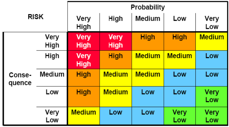
The IEC61508 standard stands for “Functional safety of electrical/electronic/programmable electronic (E/E/PE) safety-related systems” The IEC61508 standard provides a complex guideline for designing electronic systems, where the concept is based on
risk analysis,
identifying safety requirements,
design,
implementation and
validation.
Source: IEC61508 “Functional safety of electrical/electronic/programmable electronic (E/E/PE) safety-related systems”
Dependability summarizes a system’s functional reliability, meaning that a certain function is at the driver’s disposal or not. There are different aspects of dependability, first of all availability, meaning that the system should deliver the function when it is requested by the driver (e.g. the vehicle should decelerate when the driver pushes the brake pedal). The subsequent aspect is reliability, indicating that the delivered service is working as requested (e.g. the vehicle should decelerate more as the driver pushes the brake pedal more). Safety in this manner implies that the system that provides the function operates without dangerous failures. Functional security ensures that the system is protected against accidental or deliberate intrusion (this is more and more important since vehicle hacking became an issue recently [93][94][95]). There are additional important characteristics can be defined as a part of dependability like maintainability, reparability that has real add value during operation and maintenance. The figure below shows a block diagram describing the characteristics of functional dependability.
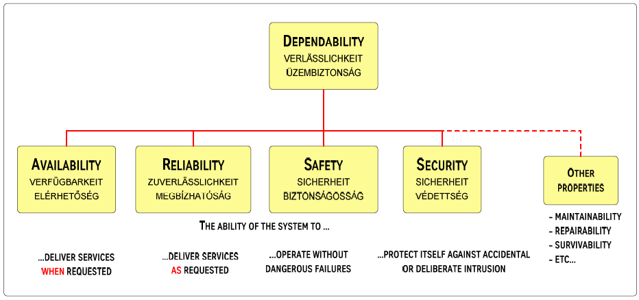
Generally the acceptable risk hazard is below the tolerable risk limit, defined by market (end-user requirements expressed by the OEMs). The probability of a function loss should be inversely related to the probability of the safety level of the function. For example in the aviation industry (Airbus A330/A340) the accepted probability of a non-intended flap control is P < 1*10-9 (Source: Büse, Diehl). Such high requirements for the availability can only be fulfilled by so called fault-tolerant systems. This is the reason why automotive safety critical systems must be fault tolerant; meaning that one failure in the system may not reduce the functionality. Please remember the two independent circuits of the traditional hydraulic brake system, having the intension that if one circuit fails, there is still brake performance (but in this case not 100%!) in the vehicle. Such systems are called 2M systems, since there are two independent mechanical circuits in the architecture.
In today’s electronically controlled safety critical systems there are usually at least one mechanical backup system. As a result, the probability of a function loss with a mechanical backup (1E+1M - one electrical system and one mechanical system architecture) can be as low as P < 1*10-8, while the probability of a function loss without mechanical backup (1E - architecture alone) is around P < 1*10-4. The objective of the safety architectural design is to provide around P < 1*10-8 level of dependability (availability) in case of 2E system architectures (electronic system with electronic backup) without mechanical backup.
Safety architectural design means consideration of all potential failures and relevant design answers to all such issues. The easiest answer to produce a fault tolerant system, so as to avoid that one failure may result is a complete function loss is to duplicate the system and extend it with arbitration logic. In case of a redundant system extended it with arbitration logic the subcomponents are not simply duplicated, but there is a coordinating control above to enable (or disable) output control based on the comparison of the two calculated outputs of the redundant subsystems. In case both subsystems have the same output (and none of them identified errors) the overall system output is enabled. Even in case of redundancy there are several tricks to enhance the safety level of a system. For example safety engineers soon realized that it makes great difference if the redundant subsystems are composed of physically the same (hardware and software) or physically different components. Early solutions just used two physically same components for redundancy, but today the different hardware and software components are predefined requirements to eliminate the systematic failures caused by design and/or software errors.
Redundancy and supervision are not only issue in case of fault tolerant architectures, safety focused approach can also be observed in ECU (electronic Control Unit) design. Early and simple ECUs were only single processor systems; while later - especially in brake system control – the dual processor architectures became widespread. Initially these two processors were the same microcontrollers (e.g. Intel C196) with the same software (firmware) inside. In this arrangement both microcontrollers have access to all of the input signals, they individually perform internal calculations based on the same algorithm each resulting in a calculated output command. These two outputs then are compared to each-other and only in case both controllers came to the same result (without any errors identified) the ECU output is controlled. This so called A-A processor architecture was a significant step forward in safety (compared to single processor systems), but safety engineers quickly understood, that this approach does not prevent system loss in case of systematic failures (e.g. microcontroller hardware bug or software implementation error). This is the reason why the A-B processor architecture was later introduced. In the A-B processor approach the two controllers physically must differ from each other. Usually the A controller is bigger and more powerful (bigger in memory capacity, having more calculation power) than the B controller. The A controller is often identified as “main” controller, while B controller is often referred to as “safety” controller, since in this task distribution the A controller is responsible for the functionality, while the B controller has only tasks for checking the A controller. B controller has access also to the inputs of the A controller, but the algorithms inside are totally different. B controller also does calculations based on the input signals, but these are not detailed calculations, only basic calculations on a higher level “like rule of thumb” checking. The different hardware and the different software algorithms in A-B processor design have proved its superior reliability.
Besides the different controller architectures there are also different kinds of dedicated supervisory electronics used extensively by the automotive electronics industry. The most significant ones are the so called “watch-dog” circuits. The watch-dogs are generally separate electronic devices that have a preset internal alarm timer. If the watch-dog does not get an “everything is OK” signal from the main controller within the predefined timeframe, the watch-dog generates a hardware reset of the whole circuitry (ECU). There are not only simple watch-dog integrated circuits available, but also more complex ones (e.g. windowed watch-dogs), however the theory of operation are basically the same.
Up to now fault-tolerant requirements were only observed from functional point-of-view, while a simple failure in the energy supply system can also easily result in function loss. That is why a fail-safe electrical energy management subsystem is a mandatory requirement for safe electrical energy supply of safety related drive-by-wire subsystems (e.g. steer-by-wire, brake-by-wire). The following figure shows a block diagram of a redundant energy management architecture (where PTC stands for Powertrain Controller, SbW stands for Steer by Wire and BbW stands for Brake by Wire subsystems).
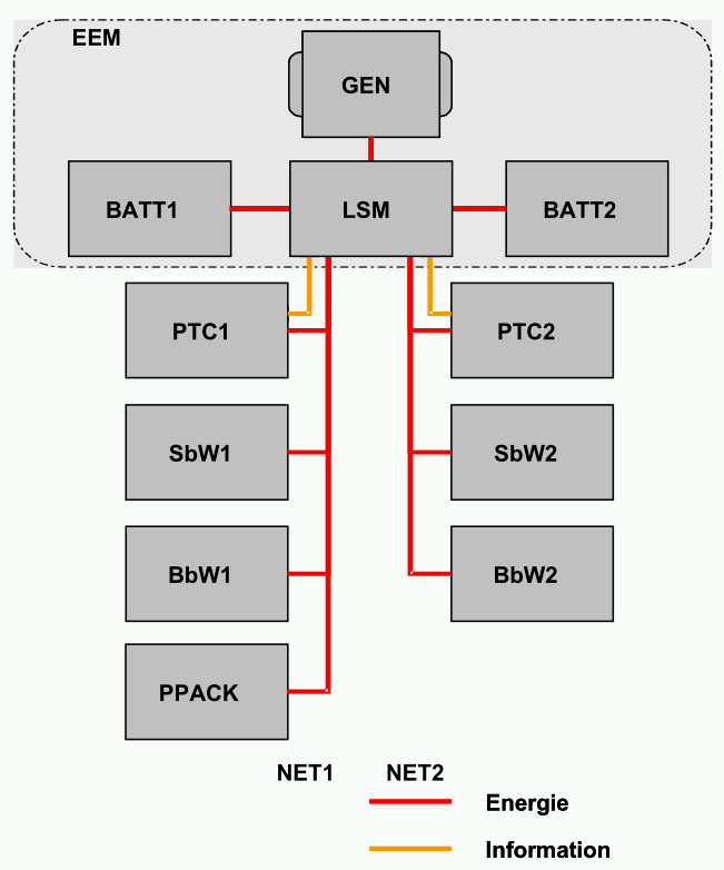
7.3. Steering
The steering system in today’s road vehicles uses mechanical linkage between the steering wheel and the steered wheels. The driver’s steering input (demand) is transmitted by a steering shaft through some type of gear reduction mechanism to generate a steering motion at the front wheels.
In the present day automobiles, power assisted steering has become a standard feature. Electrically power assisted steering has replaced the hydraulic steering aid which has been the standard for over 50 years. A hydraulic power assisted steering (HPAS) uses hydraulic pressure supplied by an engine-driven pump. Power steering amplifies and supplements the driver-applied torque at the steering wheel so that the required drive steering effort is reduced. The recent introduction of electric power assisted steering (EPAS) in production vehicles eliminates the need of the former hydraulic pump, thus offering several advantages. Electric power assisted steering is more efficient than conventional hydraulic power assisted steering, since the electric power steering motor only needs to provide assist when the steering wheel is turned, whereas the hydraulic pump must run continually. In the case of EPAS the assist level is easily adjustable to the vehicle type, road speed, and even driver preference. An added benefit is the elimination of environmental hazard posed by leakage and disposal of hydraulic power steering fluid. (Source: [96])
Although aviation industry proved that the fly-by-wire systems can be as reliable as the mechanical connection, automotive industry steps forward with intermediate phases like EPAS (electronically power assisted steering) as mentioned above and SIA (superimposed actuation) to be able to electronically intervene into the steering process.
Electric power steering (EPAS) usually consists of a torque sensor in the steering column measuring the driver’s effort, and an electric actuator which then supplies the required steering support (see Figure 104 [97]).This system enables to implement such functions that were not feasible with the former hydraulic steering like automated parking or lane departure preventions.
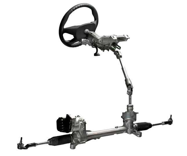
Superimposed actuation (SIA) allows driver-independent steering input without disconnecting the mechanical linkage between the steering wheel and front axle. It is based on a standard rack-and-pinion steering system extended with a planetary gear in the steering column (see Figure 105 [98]). The planetary gear has two inputs, the driver controlled steering wheel and an electronically controlled electromotor and one output connected to the steering pinion at the front axle. The output movement of the planetary gear is determined by adding the steering wheel and the electro-motor rotation. When the electromotor is not operating, the planetary gear just passes through the rotation of the steering wheel; therefore the system also has an inherent fail silent behaviour. SIA systems may provide functions like speed dependent steering and limited (nearly) steer-by-wire functionality.
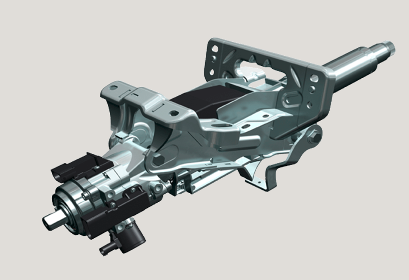
The future of driving is definitely the steer-by-wire technology. An innovative steering system allowing new degrees of freedom to implement a new human machine interface (HMI) including haptic feedback (by "cutting" the steering column, i.e. opening the mechanical connection steering wheel / steering system).
The steer-by-wire system offers the following advantages:
The absence of steering column simplifies the car interior design.
The absence of steering shaft, column and gear reduction mechanism allows much better space utilization in the engine compartment.
Without mechanical connection between the steering wheel and the road wheel, it is less likely that the impact of a frontal crash will force the steering wheel to intrude into the driver’s survival space.
Steering system characteristics can easily and infinitely be adjusted to optimize the steering response and feel.
Instead of a mechanical connection between the steering wheel and the steered axle (steering gear) the steer-by-wire system uses full electronic control. The steer-by-wire system has an electronically controlled clutch integrated into the steering rod that enables to cut or re-establish the mechanical connection in the steering system. For safety reasons this clutch can be opened by electromagnetic power, but it closes automatically (e.g. by a mechanical spring) when the electric power is missing. When the clutch is closed the steering system operates just like a “normal” mechanical steering system, where the mechanical link is continuous from the steering wheel to the steered wheels. In case the clutch is open the mechanical link no longer exists and the driver intention is detected by special sensors installed in the steering wheel. Input signal is the angle position (or steering torque) of the steering wheel, and output signal is the position of the steered wheels. The position of the steering actuator is controlled by a comparison of the desired and the actual value, which is usually measured by redundant angle sensors.
This above described solution is a 1E+1M architecture system, representing a steer-by wire system with full mechanical backup function. A similar system was installed in the PEIT demonstrator vehicle to validate steer-by-wire functionality.
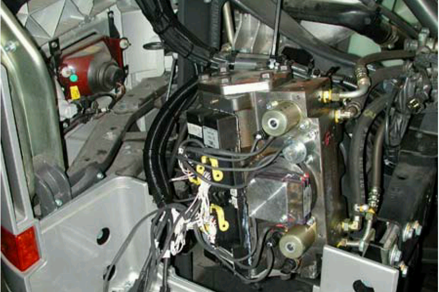
As steer-by-wire system design involves supreme safety considerations, it is not surprising that after PEIT the later HAVEit approach has extended the original safety concept with another electric control circuitry resulting in a 2E+1M architecture system. The following figure describes the safety mechanism of a steer-by-wire clutch control by introducing two parallel electronic control channels with cross checking functions [6].
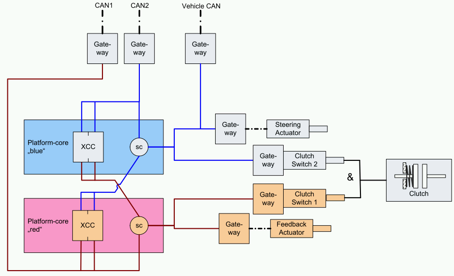
Steer-by-wire systems also raise new challenges to be resolved, like force-feedback or steering wheel end positioning. In case of the mechanical steering the driver has to apply torque to the steering wheel to turn the front wheels either to left or right directions, the steering wheel movement is limited by the end positions of the steered wheels and the stabilizer rod automatically turns back the steering wheel into the straight position. In steer-by-wire mode when the clutch is open there is no direct feedback from the steered wheels to the steering wheel and without additional components there would be no limit for turning the steering wheel in either direction. Additionally there has to be a driver feedback actuator installed in the steering wheel to provide force (torque) feedback to the driver.
Mainly due to legal legislation traced back to safety issues steer-by-wire systems are not common on today’s road vehicles however the technology to be able to steer the wheels without mechanical connection exists since the beginning of the 2000s. Up to now only Infiniti introduced a steer-by-wire equipped vehicle into the market in 2013, but its steer-by-wire system contains a mechanical backup with a fail-safe clutch described later. The Nissan system debuted under the name of Direct Adaptive Steering technology, see [99]. It uses three independent ECUs for redundancy and a mechanical backup. There is a fail-safe clutch integrated to the system, which is open during electronically controlled normal driving situations (steer-by-wire driving mode), but in case of any fault detection the clutch is closed, establishing a mechanical link from the steering wheel to the steered axle, working like a conventional, electrically assisted steering system. Figure 108 illustrates DAS system architecture with the system components.
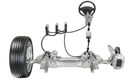
7.4. Engine
The earliest throttle-by-wire system in the automotive industry appeared on a 7 series BMW in the end of the 80s. In this case there is no mechanical Bowden coming from the accelerator pedal to the throttle valve on the engine, but there is a position sensor and a transmitter placed in the gas pedal unit, and the throttle valve is positioned by using an electric motor. A throttle-by-wire system architecture consists of a pedal module to translate the driver input to an electrical signal for the engine control module (ECM) and the electronic throttle body (ETB). The ETB receives the electrical signal command from the engine control module (ECM) and moves the throttle valve to allow airflow into engine. The ETB provides feedback of its relative position as measured by the throttle position sensor (TPS) from the throttle to the ECM.
Electronic throttle control enables the integration of features such as cruise control, traction control, stability control, pre-crash systems and others that require torque management, since the throttle can be moved irrespective of the position of the driver's accelerator pedal. Throttle-by-wire provides some benefit in areas such as air-fuel ratio control, exhaust emissions and fuel consumption reduction, and also works jointly with other technologies such as gasoline direct injection.
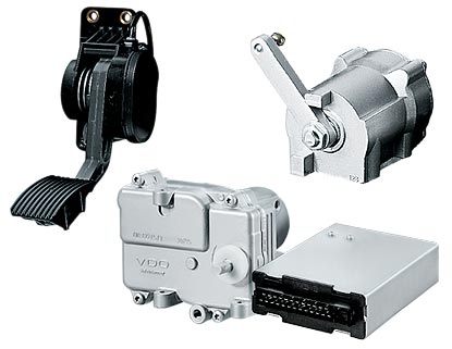
7.5. Brakes
Brake-by-wire systems were initially introduced in the heavy duty commercial vehicle segment in the mid of the 90s. The so called EBS (Electronic Brake Control) systems are rather electronically controlled pneumatic brake systems, since the energy for braking is supplied by compressed air. Ten years later in the passenger car domain Daimler and Toyota started to use such systems, with limited success. These systems are still classic hydraulic wheel brakes where the energy for braking is supplied by an electro-hydraulic pump. The greatest advantage of an electronically controlled brake system is the capability of braking each wheel according to the corresponding friction situation under the wheels. The brake-by-wire systems are fully controlled by electronic circuits and electronic/electric commands/signals. Actuation however still pneumatic in case of commercial vehicles and hydraulic in case a passenger cars. The future brake-by-wire systems may be composed of fully electronic brakes where the hydraulic system is replaced by mechatronic actuators and the energy for braking also comes from electric energy, using so called EMB (Electro-Mechanic Brake) or EWB (Electronic Wedge Brake) applications. The theory of the electronically controlled braking system is closely linked together with Prof. Egon-Christian Von Glasner who designed the first architecture of an EBS in 1987 with his partner, Micke[100].
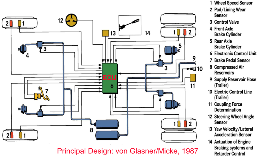
7.5.1. Electro-pneumatic Brake (EPB)
EPB stands for Electro Pneumatic Braking system, which is practically a brake-by-wire system with pneumatic actuators and pneumatic backup system. Today these systems, generally called as EBS are standard in all modern heavy duty commercial vehicles (motor vehicles and trailers). EBS was introduced by Wabco in 1996 as the series production brake system of Mercedes Benz Actros.
The basic functionality of the EBS can be observed in Figure 111 [101]. The driver presses the brake pedal which is connected to the foot brake module. It measures the pedal’s path with redundant potentiometers and sends the drivers demand to the central ECU. The EBS’s central ECU calculates the required pressure for each wheel and sends the result to the brake actuator ECUs. In this ECU there is closed loop pressure control software, which sets the air pressure in the brake chambers to the prescribed value. The actuator ECU also measures the wheel speed and sends this information back to the central EBS ECU. During the normal operation the actuator ECUs energize the so-called backup valves, which results in the pneumatic backup system’s deactivation. In case of any detected or unexpected error (and when unpowered) the backup valves are dropped and the conventional pneumatic brake system becomes active again.
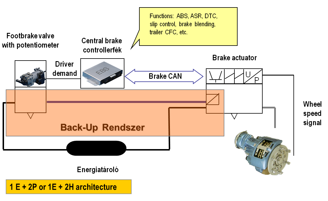
The advantages of electronic control over conventional pneumatic control are shorter response times and build-up times in brake cylinders, reducing the brake distance and the integration possibility of several active safety and comfort functions like the followings.
Anti-lock Braking System (ABS)
Traction control (ASR,TCS)
Retarder and engine brake control
Brake pad wear control
Vehicle Dynamics Control (VDC/ESP)
Yaw Control (YC)
Roll-Over Protection (ROP)
Coupling Force Control (CFC) between the tractor and semi-trailer
Adaptive Cruise Control (ACC)
Hill holder
7.5.2. Elector-hydraulic Brake (EHB)
The intention of eliminating the hydraulic connection between the brake pedal and the actuator is primarily motivated by the need of integration of the several active safety functions such as ABS, ASR and VDC (ESP).
An Electro Hydraulic Brake system is practically a brake-by-wire system with hydraulic actuators and a hydraulic backup system. Normally there is no mechanical connection between the brake pedal and the hydraulic braking system. When the brake pedal is pressed the pedal position sensor detects the amount of movement of the driver, thus the distance the brake pedal travelled. In addition the ECU feedbacks to the brake pedal’s actuator which hardens the pedal to help the driver to feel the amount of the braking force. As a function of distance the ECU determines the optimum brake pressure for each wheel and applies this pressure using the hydraulic actuators of the brake system. The brake pressure is supplied by a piston pump driven by an electric motor and a hydraulic reservoir which is sufficient for several consecutive brake events. The nominal pressure is controlled between 140 and 160 Ba. The system is capable of generating or releasing the required brake pressure in a very short time. It results in shorter stopping distance and in more accurate control of the active safety systems. Should the electronic system encounter any errors the hydraulic backup brake system is always there to take over the braking task. The following figure shows the layout of an electronically controlled hydraulic brake system[100].
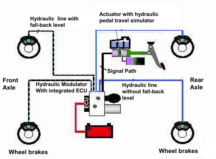
The first brake-by-wire system with hydraulic backup was born from the cooperation of Daimler and Bosch in 2001, which was called Sensotronic Brake Control (SBC). It was not a success story, because of software failures. The customers complained because the backup mode resulted in longer stopping distance and higher brake pedal effort by the driver. In May 2004, Mercedes recalled 680,000 vehicles to fix the complex brake-by-wire system. Then, in March 2005, 1.3 million cars were recalled, partly because of further unspecified problems with the Sensotronic Brake Control system. (Source: [102])
7.5.3. Electro-mechanic brake (EMB)
The EMB stands for electromechanical braking system, which is a fully brake-by-wire system. It does not use any hydraulic nor pneumatic actuators as shown on Figure 113 [100]. EMB reduces the stopping distance on account of its rapid brake response, eliminates the necessity of a brake cylinder, brake lines and hoses, as all these components are replaced by electric wiring. The use of electrics reduces maintenance expense, and also eliminates the expense of brake fluid disposal. EMB likewise measures the force of the driver's intention to brake the vehicle via sensors monitoring the system in the brake-pedal feel simulator. The ECU processes the signals received, links them where appropriate to data from other sensors and control systems, and calculates the force to be generated by the electronic brake caliper (e-caliper) of each wheel when pressing the brake pads onto the brake disc. The wheel brake modules essentially consist of an electric control unit, an electric motor and a transmission system. The electric motor and transmission system form the so-called actuator which generates the brake application forces in the brake caliper. These actuators are capable of delivering forces of up to several tons in just a few milliseconds. (Source: [103])
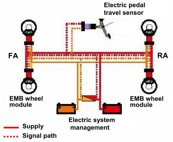
Power requirements for EMB are high and would overload the capabilities of conventional 12 volt systems installed in today's vehicles. Therefore the electro-mechanical brake is designed for a working voltage of 42 volts, which can be ensured with extra batteries.
7.6. Transmission
The torque and power of the internal combustion engine vary significantly depending on the engine revolution. The task of the transmission system mounted between the engine and the driven wheels is to adapt the engine torque according to the actual traction requirement. From highly automated driving point-of-view the automotive transmission system can be classified into two categories, namely the manual transmission and the automatic transmission. Manual transmissions cannot be integrated into a highly automated vehicle, there has to be at least an automated manual transmission or another kind of automatic transmission as will be explained later in this section.
In case of the manual transmission system, the driver has the maximum control over the vehicle; however using manual transmission requires a certain practice and experience. The manual transmission is fully mechanical system that the driver operates with a stick-shift (gearshift) and a clutch pedal. The manual transmission is generally characterized by simple structure, high efficiency and low maintenance cost.
Automatic transmission systems definitely increase the driving comfort by taking over the task of handling the clutch pedal and choosing the appropriate gear ratio from the driver. Regardless of the realization of the automatic transmission system, the gear selection and changing is done via electronic control without the intervention of the driver. There are different types of automatic transmission systems available, like
Automated Manual Transmission (AMT)
Dual Clutch Transmission (DCT/DSG)
Hydrodynamic Transmission (HT)
Continuously Variable Transmission (CVT)
7.6.1. Clutch
The purpose of the clutch is to establish a releasable torque transmission link between the engine and the transmission through friction, allowing the gears to be engaged. Besides changing gears it enables functions like smooth starting of the vehicle or stopping the car without having to stop the internal combustion engine. In traditional vehicles the clutch is operated by the driver through the clutch pedal that uses mechanical Bowden or a hydraulic link to the clutch mechanism. In clutch-by-wire applications there is no need for a clutch pedal, the release and engage of the clutch is controlled by an electronic system.
In the SensoDrive electronically controlled manual transmission system of Citroen there is no clutch pedal. The gear shifting is simply done by selecting the required gear with the gear stick or the paddle integrated into the steering wheel. During gear shifting the driver even does not have to release the accelerator pedal. The SensoDrive system is managed by an electronic control unit (ECU), which controls two actuators. One actuator changes gears while the other, which is equipped with a facing wear compensation system, opens and closes the clutch. The following figure illustrates the operation of the clutch-by-wire system of Citroen [104].
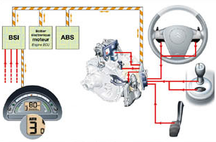
7.6.2. Automated Manual Transmission (AMT)
In case of an automated manual transmission (AMT) a simple manual transmission is transformed into an automatic transmission system by installing a clutch actuator, a gear selector actuator and an electronic control unit. The shift-by-wire process is composed of the following steps. After the clutch is opened by the electromechanical clutch actuator, the gear shifting operation in the gearbox is carried out by the electromechanical transmission actuator. When the appropriate gear is selected then the electromechanical clutch actuator closes the clutch and drive begins. These two actuators are controlled by an electronic control unit. If required, the system determines the shift points fully automatically, controls the shift and clutch processes, and cooperates with the engine management system during the shift process with respect to engine revolution and torque requests [105].
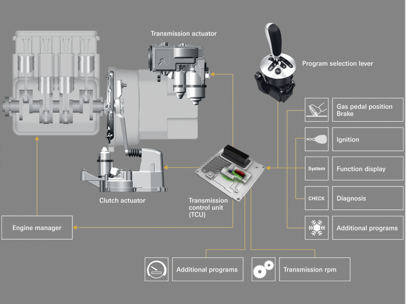
Automated Manual Transmissions have a lot of favourable properties; the disadvantage is that the power flow (traction) is lost during switching gear, as it is necessary to open the clutch. This is what automatic transmission systems have eliminated providing continuous traction during acceleration.
7.6.3. Dual Clutch Transmission (DTC/DSG)
The heart of the Dual Clutch Transmission (DCT) is the combined dual clutch system. The DSG acronym is originally derived from the German word of “DoppelSchaltGetriebe” but it also has an English alternative of “Direct Shift Gearbox”. The reason for the naming is that there are two transmission systems integrated into one. Transmission one includes the odd gears (first, third, fifth and reverse), while transmission two contains the even gears (second, fourth and sixth). The combined dual clutch system switches from one to the other very quickly, releasing an odd gear and at the same time engaging a preselected even gear and vice versa. Using this arrangement, gears can be changed without interrupting the traction from the engine to the driven wheels. This allows dynamic acceleration and extremely fast gear shifting times that are below human perception[106].
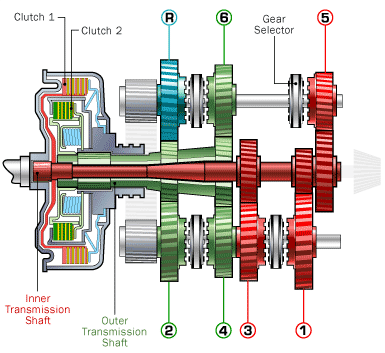
7.6.4. Hydrodynamic Transmission (HT)
The hydrodynamic torque converter and planetary gear transmissions can be found in premium segment passenger cars, commercial vehicles and buses. The design of the hydrodynamic transmission with planetary gear is simple and clear as can be observed on the figure below[107]. The main piece is the hydrodynamic counter-rotating torque converter. Situated in front of it are the impeller brake, the direct gear clutch, the differential transmission, the input clutch and the overdrive clutch. A hydraulic torsional vibration damper at the transmission input reduces engine vibrations effectively. Behind the converter, an epicyclical gear combines the hydrodynamic and mechanical forces. The final set of planetary gears activates the reverse gear and, during braking, also the retarder Gear-shifting commands are placed by the electronic control system; gear shifting occurs electro-hydraulically, with solenoid valves. The transmission electronic control unit is in continuous data exchange with other ECUs like engine and the brake system management to provide a harmonized control.
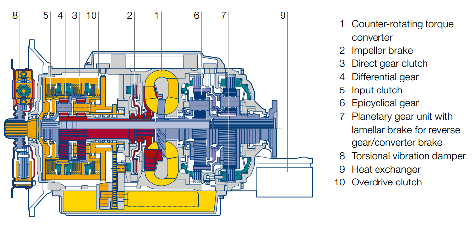
7.6.5. Continuously Variable Transmission (CVT)
The Continuously Variable Transmission (CVT) ideally matches the needs of vehicle traction. This is also beneficial in terms of fuel consumption, pollutant emissions, acceleration and driving comfort. The first series production CVT appeared in 1959 in a DAF city car, but technology limitations made it suitable for engines with less than 100 horsepower. The enhanced versions with electronic control capable of handling more powerful engines can be found in the production line of several major OEM.
While traditional automatic transmissions use a set of gears that provides a given number of ratios there are no gears in CVT transmissions, but two V-shaped variable-diameter pulleys connected with a metal belt. One pulley is connected to the engine, the other to the driven wheels.
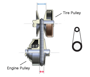
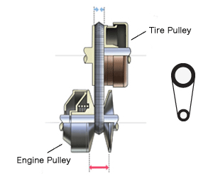
Changing the diameter of the pulleys varies the transmission ratio (the number of times the output shaft spins for each revolution of the engine). Illustrated in the figures above, as the engine (input) pulley width increases and the tire (output) pulley width decreases, the engine pulley becomes smaller than the tire pulley for the diameter of the part where the pulley and the belt are in contact. This is the state of being in low gear. Vice versa, as the engine pulley width decreases and the tire pulley width increases, the diameter of the part where belt and pulley are in contact grows larger for the engine pulley than the tire pulley, which is the state of being in high gear. The main advantage of the CVT is that pulley width can be continuously changed, allowing the system to change transmission gear ratio smoothly and without steps [108].
The controls for a CVT are the same as an automatic: Two pedals (accelerator and brake) and a P-R-N-D-L-style shift pattern.
Chapter 8. Vehicle to Vehicle interactions (V2V)
Nowadays the developed countries are increasingly characterized by a pervasive computing environment. The people’s living environments are emerging based upon information resource provided by the connections of various communication networks. New handheld devices like smartphones and tablets enhance information processing and global access of users. During the last decade, advances in both hardware and software technologies have resulted in the need for connecting the vehicles with each other. In this chapter first the basic theory of the Mobile Ad Hoc Networks are introduced, then the available functions and the advantages of the vehicle to vehicle interactions are detailed.
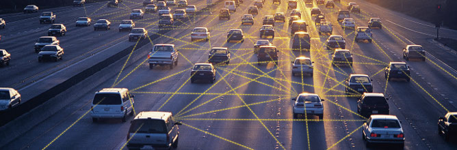
8.1. Mobile Ad Hoc Network Theory
Mobile networking is one of the most important technologies supporting pervasive computing, and it is the essential technology for the vehicular ad-hoc network development. The basic theory of MANETs is discussed based on the PhD thesis in [109].
Generally there are two distinct approaches for enabling wireless mobile units to communicate with each other: infrastructure-based and ad hoc.
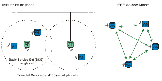
Wireless mobile networks have traditionally been based on the cellular concept and relied on good infrastructure support, in which mobile devices communicate with access points (or base stations) connected to the fixed network infrastructure. Typical examples of this kind of wireless networks are GSM, UMTS, WLL, WLAN, etc.
In recent years the widespread availability of wireless communication and handheld devices has stimulated research on self-organizing networks that do not require a pre-established infrastructure. These ad hoc networks consist of autonomous nodes that collaborate in order to transfer information. Usually these nodes act as end systems and routers at the same time. Ad hoc networks can be subdivided into two classes: static and mobile. In static ad hoc networks the position of a node may not change once it has become part of the network.
In mobile ad hoc networks, systems may move arbitrarily. A Mobile Ad Hoc Network is commonly called a MANET. Mobile Ad Hoc Networks creates the basis for connectivity between vehicles which is called Vehicular Ad Hoc Network. It is a variation of MANETs, with the emphasis being now the node is the vehicle.
A MANET is a collection of wireless mobile nodes that dynamically form a network to exchange information without using any pre-existing fixed network infrastructure or a centralized administration. MANET nodes are equipped with wireless transmitters and receivers using antennas, which may be omni-directional (broadcast), highly -directional (point-to-point), possibly steerable, or some combination thereof. At a given point in time depending on the nodes’ positions and their transmitter and receiver coverage patterns, transmission power levels and co-channel interference levels, a wireless connectivity in the form of a random, multi-hop graph or ad hoc network formulates between the nodes. This ad hoc topology may change with time as the nodes move or adjust their transmission and reception parameters.
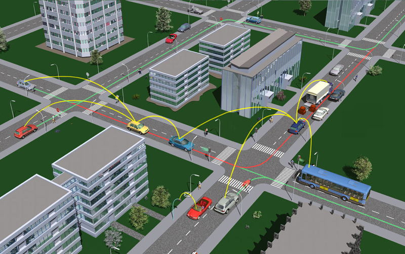
In such an environment, it may be necessary for one mobile host to use the aid of other hosts in forwarding a packet to its destination, due to the limited range of each mobile host’s wireless transmissions.
MANETs are a very important part of communication technology that supports truly pervasive computing, because in many contexts information exchange between mobile units cannot rely on any fixed network infrastructure, but on rapid configuration of wireless connection. Next generation of mobile communications will include both infrastructure wireless networks and infrastructureless Mobile Ad Hoc Networks (MANETs).
The special features of MANET bring this technology great opportunity together with severe challenges. Since mobile ad hoc networks change their topology frequently and without prior notice, routing in such networks is a challenging task. A MANET is some way like an autonomous system in which mobile hosts connected by wireless links are free to move randomly and often act as routers at the same time.
The traffic types in ad hoc networks are quite different from those in an infrastructure wireless network, including:
Peer-to-Peer. Communication between two nodes that are within one hop. Network traffic is usually consistent.
Remote-to-Remote. Communication between two nodes beyond a single hop but which maintain a stable route between them. This may be the result of several nodes staying within communication range of each other in a single area or possibly moving as a group. The traffic is similar to standard network traffic.
Dynamic Traffic. This occurs when nodes are dynamic and moving around. Routes must be reconstructed. This results in a poor connectivity and network activity in short bursts.
A MANET has the following special characteristics (See [109] and [110]).
Autonomous terminal. In a MANET, each mobile terminal is an autonomous node, which may function as both a host and a router. In other words, besides the basic processing ability as a host, the mobile nodes can also perform switching functions as a router. So usually endpoints and switches are indistinguishable in MANET.
Distributed operation. Since there is no background network for the central control of the network operations, the control and management of the network is distributed among the terminals. The nodes involved in a MANET should collaborate amongst themselves and each node acts as a relay as needed, to implement functions e.g. security and routing.
Dynamic network topology. Since the nodes are mobile, the network topology (which is typically multi-hop) may change rapidly and unpredictably and the connectivity among the terminals may vary with time. MANET should adapt to the traffic and propagation conditions as well as the mobility patterns of the mobile network nodes. The mobile nodes in the network dynamically establish routing among themselves as they move about, forming their own network on the fly. Moreover, a user in the MANET may not only operate within the ad hoc network, but may require access to a public fixed network.
Multi-hop routing. Basic types of ad hoc routing algorithms can be single -hop and multi-hop, based on different link layer attributes and routing protocols. Single-hop MANET is simpler than multi-hop in terms of structure and implementation, with the cost of less functionality and applicability. When delivering data packets from a source to its destination out of the direct wireless transmission range, the packets should be forwarded via one or more intermediate nodes.
Bandwidth-constrained, fluctuating capacity links. The nature of high bit-error rates of wireless connection might be more profound in a MANET. One end-to-end path can be shared by several sessions. The channel over which the terminals communicate is subject to noise, fading, and interference, and has less bandwidth than a wired network. In some scenarios, the path between any pair of users can traverse multiple wireless links and the link themselves can be heterogeneous. One effect of the relatively low to moderate link capacities is that congestion is typically the norm rather than the exception, i.e. aggregate application demand will likely approach or exceed network capacity frequently.
Energy and processing constrained operation. In most cases, the MANET nodes are mobile devices with less CPU processing capability, small memory size, and low power storage compared to desktop or fixed devices. Such devices need optimized algorithms and mechanisms that implement the computing and communicating functions.
Limited physical security: Mobile wireless networks are generally more disposed to physical security threats than are fixed-cable nets. The increased possibility of eavesdropping, spoofing, and denial-of-service attacks should be carefully considered. Existing link security techniques are often applied within wireless networks to reduce security threats. As a benefit, the decentralized nature of network control in MANETs provides additional robustness against the single points of failure of more centralized approaches.
Summarizing a mobile ad hoc network is a collection of autonomous mobile nodes that form a dynamic, purpose-specific, multi-hop radio network in a decentralized manner. The nature of such networks is the absence of a fixed support infrastructure (such as mobile switching centres, base stations, access points) traditionally seen in wireless networks. The network topology is constantly changing as a result of nodes joining in and moving out. Packet forwarding, routing, and other network operations are carried out by the individual nodes themselves. The features of MANET introduce several challenges which are detailed in the following subsections.
8.1.1. Routing
Since the topology of the network is constantly changing, the issue of routing packets between any pair of nodes becomes a challenging task. In a MANET routers (i.e. hosts) can be mobile and inter -router connectivity can change frequently during normal operation. In contrast the Internet (like most of the telecom networks) possesses a quasi-fixed infrastructure consisting of routers or switches that forward data over hardwired links. Traditionally end-user devices, such as host computers or telephones, attach to these networks at fixed locations. As a consequence they are assigned addresses based on their location in a fixed network-addressing hierarchy. It simplifies routing in these systems, as a user’s location does not change.
The end devices are increasingly mobile, meaning that they can change their point of attachment to the fixed infrastructure. This is the paradigm of cellular telephony and its Internet equivalent, mobile data network. In this approach a user’s identity depends upon whether the user adopts a location-dependent (temporary) or location-independent (permanent) identifier. Users with temporary identifiers are sometimes referred to as nomadic, whereas users with permanent identifiers are referred to as mobile. The distinction is that although nomadic users may move, they carry out most network related functions in a fixed location. Mobile users must work “on the go” changing points of attachment as necessary. In either case additional networking support may be required to track a user’s location in the network so that information can be forwarded to its current location using the routing support within the more traditional fixed hierarchy.
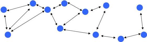
Internet is hardly tuned to allow mobility during the data transfers because protocols are not conceived for devices that frequently change their point of attachment in the topology. There is typically a change of the physical IP address each time a mobile node changes its point of attachment and thus its reachability to the Internet topology. This results in losing packets in transit and breaking transport protocols connections if mobility is not handled by specific services. The protocol stack must therefore be upgraded with the ability to cross networks during data transfers, without breaking the communication session and with minimum transmission delays and signalling overhead. This is commonly referred to as mobility support. Host mobility support is handled by Mobile IPv6.
In contrast, the goal of mobile ad hoc networking is to extend mobility into the field of autonomous, mobile, wireless domains, where a set of nodes, which may be combined routers and hosts, themselves form the network routing infrastructure in an ad hoc way. With Mobile Ad Hoc Networking, the routing infrastructure can move along with the end devices. Thus the infrastructure’s routing topology can change, and the addressing within the topology can change. In this paradigm an end-user’s association with a mobile router (its point of attachment) determines its location in the MANET. As mentioned above a user’s identity may be temporary or permanent. The fundamental differences in the composition of the routing infrastructure (fixed, hardwired, and bandwidth-rich opposite to dynamic, wireless, and bandwidth-constrained) causes that much of the fixed infrastructure’s control technology is no longer useful. The infrastructure’s routing algorithms and much of the networking suite must be reworked to function efficiently and effectively in mobile environment.
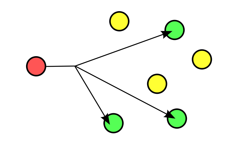
Multicast routing (delivery of information to a group of destination devices simultaneously in a single transmission) is another challenge because the multicast tree is no longer static due to the random movement of nodes within the network. Routes between nodes may potentially contain multiple hops, which is more complex than the single hop communication.
8.1.2. Security
In addition to the common vulnerabilities of wireless connection an ad hoc network has its particular security problems. Mobile hosts join in on the fly and create a network on their own. With the network topology changing dynamically and the lack of a centralized network management functionality, these networks tend to be vulnerable to a number of attacks. If such networks are to succeed in the transportation, the security aspect naturally assumes importance. The unreliability of wireless links between nodes, constantly changing topology owing to the movement of nodes in and out of the network and lack of incorporation of security features in statically configured wireless routing protocols not meant for ad hoc environments all lead to increased vulnerability and exposure to attacks.
Security in wireless ad hoc networks is particularly difficult to achieve, because of the vulnerability of the links, the limited physical protection of each of the nodes, the sporadic nature of connectivity, the dynamically changing topology, and the absence of a certification authority and the lack of a centralized monitoring or management point. This underscores the need for intrusion detection, intrusion prevention, and related countermeasures. The wireless links between nodes are highly susceptible to link attacks, which include the following threats (See [111]).
Passive eavesdropping
Active interfering
Leakage of secret information
Data tampering
Impersonation
Message replay or distortion
Denial of service (DoS)
Eavesdropping might give an adversary access to secret information, violating confidentiality. Active attacks might allow the adversary to delete messages, to inject erroneous messages, to modify messages, and to impersonate a node, thus violating availability, integrity, authentication, and non-repudiation (these and other security needs are discussed in the next section). Ad hoc networks do not have a centralized piece of machinery such as a name server, which could lead to a single point of failure and thus, make the network that much more vulnerable.
An additional problem related to the compromised nodes is the potential byzantine failures encountered within Mobile Ad hoc Network (MANET) routing protocols wherein a set of the nodes could be compromised in such a way that the incorrect and malicious behaviour cannot be directly noted at all. The compromised nodes may seemingly operate correctly, but, at the same time, they may make use of the flaws and inconsistencies in the routing protocol to undetectably distort the routing fabric of the network. In addition such malicious nodes can also create new routing messages and advertise non-existent links, provide incorrect link state information and flood other nodes with routing traffic, thus inflicting byzantine failures on the system. Such failures are severe, because they may come from seemingly trusted nodes. Even if the compromised nodes were noticed and prevented from performing incorrect actions, the erroneous information generated by the byzantine failures might have already been propagated through the network.
Finally scalability is another issue that has to be addressed when security solutions are being devised, for the simple reason that an ad hoc network may consist of hundreds or even thousands of nodes. The scalability requirements directly affect the scalability requirements targeted to various security services such as key management. Standard security solutions would not be good enough since they are essentially for statically configured systems. This gives rise to the need for security solutions that adapt to the dynamically changing topology and movement of nodes in and out of the network.
These vulnerabilities allow a lot of special attacks in the vehicular networks including but not limited to the following examples:
Bogus information (Figure 124): Attackers diffuse wrong information in the network to affect the behaviour of other drivers (e.g., to divert traffic from a given road and thus free it for themselves).
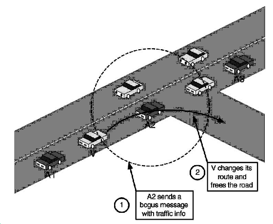
Cheating with sensor information: Attackers in this case use this attack to alter their perceived position, speed, direction, etc. in order to escape liability, notably in the case of an accident. In the worst case, colluding attackers can clone each other and having full trust between the attackers.
ID disclosure of other vehicles in order to track their location. This is the “Big Brother” scenario, where a global observer can monitor trajectories of targeted vehicles and use this data for a range of purposes (e.g., the way some car rental companies track their own cars). To monitor the global observer can leverage on the roadside infrastructure or the vehicles around its target (e.g., by using a virus that infects neighbours of the target and collects the required data).
Denial of Service: The attacker may want to bring down the VANET or even cause an accident. Example attacks include channel jamming and aggressive injection of dummy messages.
Masquerading: The attacker actively pretends to be another vehicle by using false identities and can be motivated by malicious or rational objectives.
As apparent from the above the security aspects are the most critical challenges before the wide spreading of the vehicular networks.
8.1.3. Quality of Service (QoS)
The goal of QoS support is to achieve a more deterministic communication behaviour, so that information carried by the network can be better prioritized and network resources can be better utilized. The notion of QoS is an agreement or a guarantee by the network to provide a set of measurable pre-specified service attributes to the user in terms of network delay, delay variance (jitter), available bandwidth, probability of packet loss (loss rate), etc. The IETF RFC 2386 characterizes QoS as a set of service requirements to be met by the network while transporting a packet stream from source to destination. A network’s ability to provide a specific QoS depends upon the properties of the network itself, which span over all the elements in the network. For the transmission link, the properties include link delay, throughput, loss rate, and error rate. For the nodes, the properties include hardware capability, such as processing speed and memory size. Above the physical qualities of nodes and transmission links, the QoS control algorithms operating at different layers of the network also contribute to the QoS support in networks. Unfortunately the features of MANETs show weak support for QoS. The wireless link has low, time-varying raw transmission capacity with relatively high error rate and loss rate. In addition, the possible various wireless physical technologies that nodes may use simultaneously to communicate make MANETs heterogeneous in nature. Each technology will require a MAC layer protocol to support QoS. Therefore the QoS mechanisms above the MAC layer should be flexible to fit the heterogeneous underlying wireless technologies. Providing different quality of service levels in a constantly changing environment will be a challenge. The inherent stochastic feature of communications quality in a MANET makes it difficult to offer fixed guarantees on the services offered to a device.
8.1.4. Internetworking
In addition to the communication within an ad hoc network, internetworking between MANET and fixed networks (mainly IP based) is often expected in many cases. The coexistence of routing protocols in such a mobile device is a challenge for the harmonious mobility management.
8.1.5. Power Consumption
For most of the light-weight (handheld) mobile terminals and also the built-in automotive ECUs, the communication-related functions should be optimised for low power consumption. Conservation of power and power-aware routing must be taken into account.
8.2. V2V standards
Three categories of standards deal with the vehicular networks. The IEEE 802.11 standard body is currently working on a new amendment, IEEE 802.11p, to satisfy the above mentioned requirements. This document is named Wireless Access in Vehicular Environment, also known as WAVE.
As shown in Figure 125 [112] IEEE 802.11p WAVE is only a part of a group of standards related to all layers of protocols for V2V operations. The IEEE 802.11p standard is limited by the scope of IEEE 802.11, which is strictly a MAC and PHY level standard that is meant to work within a single logical channel.
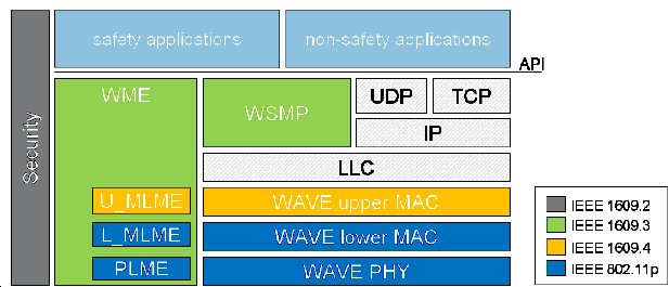
All knowledge and complexities related to the V2V operational concept are taken care of by the upper layer IEEE 1609 standards. It is intended to operate with IEEE 802.11p.
The third standard is developed by the Society of Automotive Engineers (SAE). Their J2735 standard can be placed in the application layer. It defines message sets, data frames and elements which are used for V2V and V2I safety exchanges.
8.2.1. IEEE 802.11p (WAVE)
The IEEE 802.11p WAVE standardization process originates from the allocation of the Dedicated Short Range Communications (DSRC) spectrum band in the United States and the effort to define the technology for usage in the DSRC band. The evolutions and the basics are explained in the following chapters from [112].
In 1999 the U.S. Federal Communication Commission allocated 75MHz of Dedicated Short Range Communications (DSRC) spectrum at 5.9 GHz to be used exclusively for vehicle-to-vehicle and infrastructure-to-vehicle communications. The primary goal is to enable public safety applications that can save lives and improve traffic flow. Private services are also permitted in order to spread the deployment costs and to encourage the quick development and adoption of DSRC technologies and applications.
As shown in Figure 126 the DSRC [113] spectrum is structured into seven 10 MHz wide channels. Channel 178 is the control channel (CCH), which is restricted to safety communications only. The two channels at the ends of the spectrum band are reserved for special uses. The rest are service channels (SCH) available for both safety and non-safety usage.
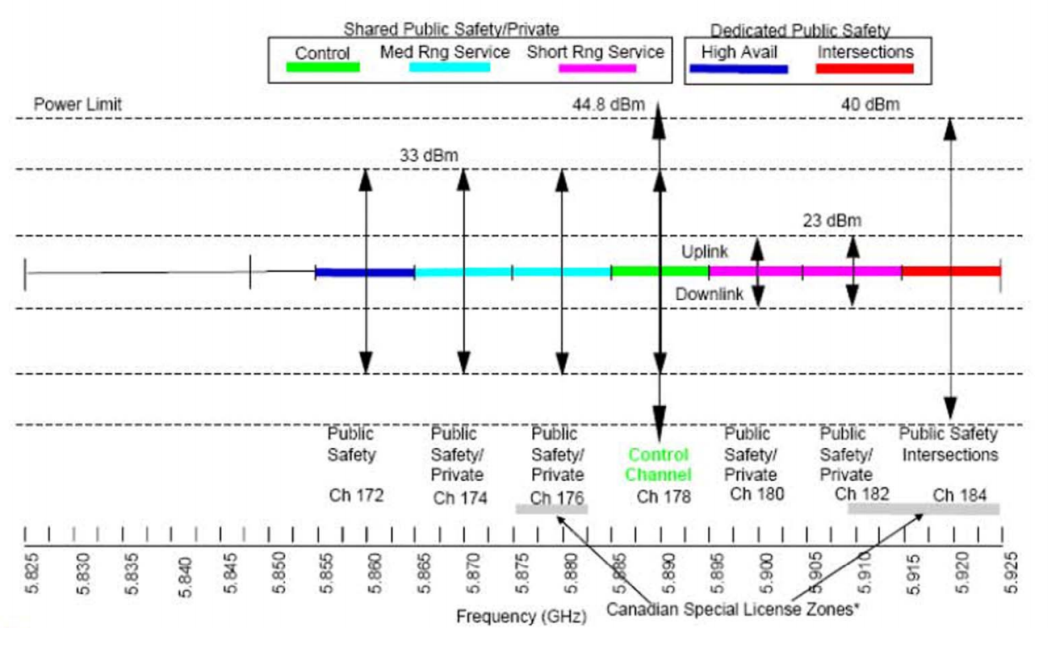
The DSRC band is a free but licensed spectrum. It is free because the Federal Communications Commission (FCC) does not charge a fee for the spectrum usage. Yet it should not be confused with the unlicensed bands in 900 MHz, 2.4 GHz and 5 GHz that are also free in usage. These unlicensed bands, which are increasingly populated with WiFi, Bluetooth and other devices, place no restrictions on the technologies other than some emission and co-existence rules. The DSRC band, on the other hand, is more restricted in terms of the usages and technologies. FCC rulings regulate usage within certain channels and limit all radios to be compliant to a standard. In other words one cannot develop a different radio technology (e.g. that uses all 75 MHz of spectrum) for usage in the DSRC band even if it is limited in transmission power as related to the unlicensed band.
Similar efforts are occurring in Europe to set spectrum aside for vehicular usage. Since 2008 European Commission’s decision provides a single EU-wide frequency band that can be used for immediate and reliable communication between cars, and between cars and roadside infrastructure. It is 30 MHz of spectrum in the 5.9 Gigahertz (GHz) band which is allocated by national authorities across Europe to road safety applications, without barring other services already in place (such as radio amateur services). The intention is that compatibility with the USA will be ensured even if the allocation is not exactly the same; frequencies will be sufficiently close to enable the use of the same antenna and radio transmitter/receiver. (Source: [114])
The worldwide DSRC spectrum allocation is shown in Figure 127 [113].
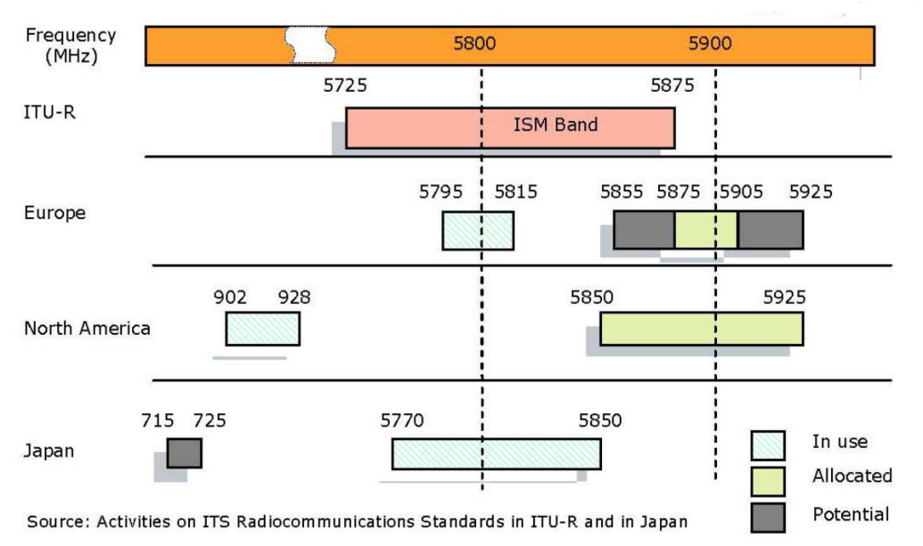
In the U.S. the initial effort at standardizing DSRC radio technology took place in an American Society for Testing and Materials (ASTM) working group. In particular the FCC rule and order specifically referenced this document for DSRC spectrum usage rules. In 2004 this effort migrated to the IEEE 802.11 standard group as DSRC radio technology is essentially IEEE 802.11a adjusted for low overhead operations in the DSRC spectrum. Within IEEE 802.11 DSRC is known as IEEE 802.11p WAVE. IEEE 802.11p is not a standalone standard. It is intended to amend the overall IEEE 802.11 standard.
One particular implication of moving the DSRC radio technology standard into the IEEE 802.11 space is that now WAVE is fully intended to serve as an international standard applicable in other parts of the world as well as in the U.S. The IEEE 802.11p standard is meant to:
Describe the functions and services required by WAVE-conformant stations to operate in a rapidly varying environment and exchange messages without having to join a Basic Service Set (BSS), as in the traditional IEEE 802.11 use case.
Define the WAVE signalling technique and interface functions that are controlled by the IEEE 802.11 MAC.
8.2.2. IEEE 1609
The IEEE 1609 family of standards defines the following parts (see [113]):
architecture,
communication model,
management structure,
security mechanisms and
physical access for high speed (<27 Mb/s), short range (<1000m) and low latency wireless communications in the vehicular environment.
The primary architectural components defined by these standards are the On Board Unit (OBU), Road Side Unit (RSU) and WAVE interface.
The IEEE 1609.3 standard covers the WAVE connection setup and management. The IEEE 1609.4 standard sits right on top of the IEEE 802.11p and enables operation of upper layers across multiple channels, without requiring knowledge of PHY parameters. The standards also define how applications that utilize WAVE will function in WAVE environment. They provide extensions to the physical channel access defined in WAVE.
8.2.3. SAE J2735
The third important standard related to vehicle communication is the J2735, Dedicated Short Range Communications (DSRC) Message Set Dictionary, maintained by the Society of Automotive Engineershttp://www.sae.org). This SAE Standard specifies a message set, its data frames and data elements specifically for use by applications intended to utilize the (DSRC/WAVE) communications systems. Although the scope of this Standard is focused on the message set and data frames of DSRC. This standard therefore specifies the definitive message structure and provides sufficient background information for the proper interpretation of the message definitions from the point of view of an application developer implementing the messages according to the DSRC standards.
It supports interoperability among DSRC applications through the use of standardized message sets, data frames and data elements. The message sets specified in J2735 define the message content delivered by the communication system at the application layer and thus defines the message payload at the physical layer. The J2735 message sets depend on the lower layers of the DSRC protocol stack to deliver the messages from applications at one end of the communication system (OBU of the vehicle) to the other end (a roadside unit). The lower layers are addressed by IEEE 802.11p, and the upper layer protocols are covered in the IEEE 1609.x series of standards.
The message set dictionary contains:
15 Messages
72 Data Frames
146 Data Elements
11 External Data Entries
The most important message type is the basic safety message (often informally called “heartbeat” message because it is constantly being exchanged with nearby vehicles). Frequent transmission of “heartbeat” messages extends the vehicle’s information about the nearby vehicles complementing autonomous vehicle sensors. Its major attributes are the following [115]:
Temporary ID
Time
Latitude
Longitude
Elevation
Positional Accuracy
Speed and Transmission
Heading
Acceleration
Steering Wheel Angle
Brake System Status
Vehicle Size
The other kinds of messages are the following (See [113]):
A la carte message ‐‐ composed entirely of message elements determined by the sender, allowing for flexible data exchange.
Emergency vehicle alert message ‐‐ used for broadcasting warnings to surrounding vehicles that an emergency vehicle is operating in the vicinity.
Generic transfer message ‐‐ provides a basic means to exchange data across the vehicle‐to‐roadside interface.
Probe vehicle data message ‐‐ contains status information about the vehicle to enable applications that examine traveling conditions on road segments.
Common safety request message ‐‐ used when a vehicle participating in the exchange of the basic safety message can make specific requests to other vehicles for additional information required by safety applications.
8.3. V2V applications
V2V communication enables a great number of use cases mostly in relation to improve driving safety or traffic efficiency and provide information or entertainment to the driver. The definitions of the below mentioned use cases are based on CAR 2 CAR Communication Consortium Manifesto [116].
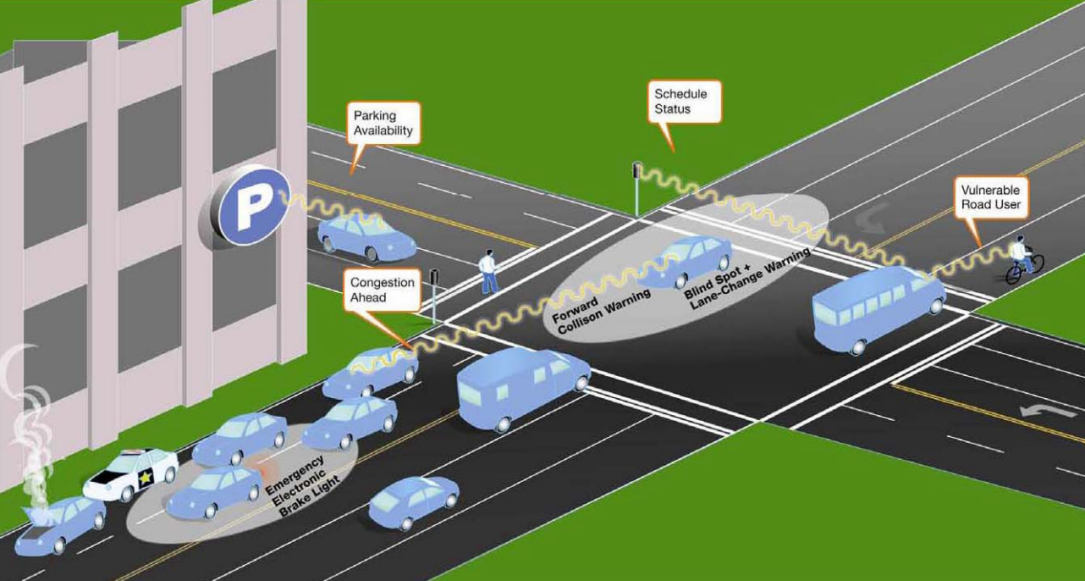
8.3.1. Traffic Safety
Safety use cases are those where a safety benefit exists when the vehicle enters into a scenario applicable to the use case. The following safety applications can be relevant with the help of V2V communication.
Warnings on entering intersections or departing highways
Hazardous location warning: obstacle discovery, reporting accidents
Sudden stop warnings: forward collision warning, pre-crash sensing or warning
Lane change/keeping warnings/assistance
Privileging ambulances, fire trucks, and police cars
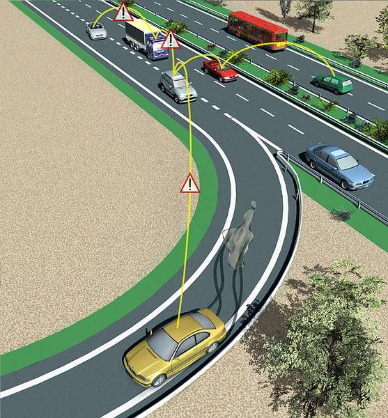
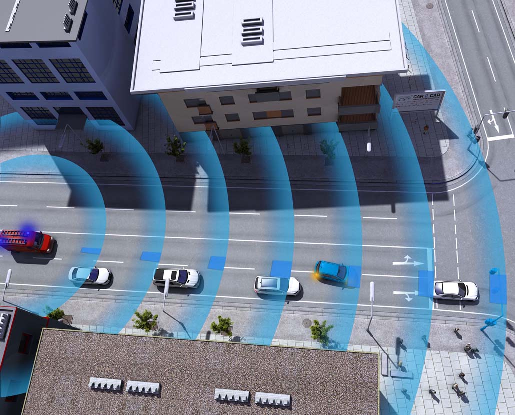
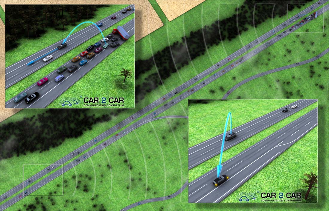
8.3.2. Traffic Efficiency
Traffic Efficiency use cases are those meant to improve efficiency of the transportation network by providing information either to the owners of the transportation network or to the drivers on the network.
Enhanced Route Guidance and Navigation
Intelligent intersections: Adaptable traffic lights, Automated traffic intersection control, Green Light Optimal Speed Advisory
Merging Assistance: enters an on-ramp to a limited access roadway (it is also a safety application)
Variable speed limits
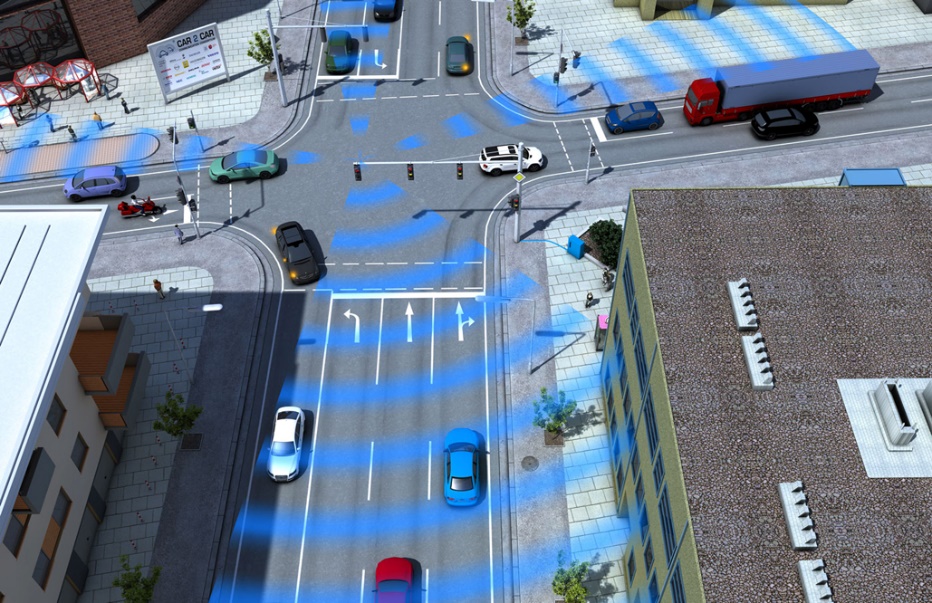
8.3.3. Infotainment and payments
This category does not contain direct traffic related applications, rather comfort services. Many of these use cases interact more directly with the vehicle owner on daily basis providing entertainment or information on a regular basis. Others are transparent to the driver but still perform a valuable function such as increasing fuel economy.
The electronic payment applications result in convenient payments and avoiding congestions caused by toll collection and makes pricing more manageable and flexible.
Internet access
POI notification
Toll collecting
Parking payment
8.3.4. Other applications
The V2V communication system can support the currently available driver assistance systems. With help of the broadcasted vehicle parameters the adaptive cruise control and park pilot functions can be improved.
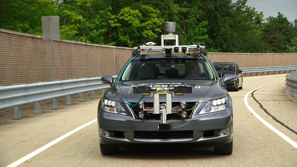
With special low-cost roadside units (RSU) the road sign recognition function can be supported and the reliability can be improved. In special cases it could offer safety functions in case of bridge or tunnel height or gate width.
Another important field of usage could be the policing and enforcement. Police could use the V2V communication in several ways especially checking the traffic rules such as:
Surveillance (e.g. finding stolen vehicles)
Speed measurements
Pull-over commands
Red light drive through
Restricted entries
Chapter 9. Vehicle to Infrastructure interaction (V2I)
The Vehicle to Infrastructure interaction, similarly to V2V, is based on wireless communication technologies. The V2I communication (commonly called V2X) is also an extensively researched topic in the United States. The main traffic safety goals of such systems are well summarized by USDOT's (U.S. Department of Transportation) Connected Vehicles Program [117]. V2I is the wireless exchange of critical safety and operational data between vehicles and highway infrastructure, intended primarily to avoid or mitigate motor vehicle accidents but also to enable a wide range of other safety, mobility, and environmental benefits. V2I communications apply to all vehicle types and all roads, and transform infrastructure equipment into “smart infrastructure”. They incorporate algorithms that use data exchanged between vehicles and infrastructure elements to perform calculations that recognize high-risk situations in advance, resulting in driver alerts and warnings through specific actions. One particularly important advantage is the ability for traffic signal systems to communicate the signal phase and timing (SPAT) information to the vehicle in support of delivering active safety advisories and warnings to drivers.
9.1. Architecture
Several V2I architectures can be found in the different research papers. But generally these systems consist of the same key components, on the basis of which a general framework can be defined. Such an architecture framework was defined by USDOTs’ ITS Joint Program Office. The minimal V2I system should contain the following parts:
Vehicle On-Board Unit or Equipment (OBU or OBE)
Roadside Unit or Equipment (RSU or RSE)
Safe Communication Channel
The OBUs are the vehicle side of the V2I system. Practically the same physical device as for the V2V communication. In this document, references to the OBUs are used to describe the functions performed within the vehicle in addition to the radio transmission element. An OBU is logically composed of a radio transceiver (typically DSRC), a GPS system, an applications processor and interfaces to vehicle systems and the vehicle’s human machine interface (HMI). OBUs provide the communications both between the vehicles and the RSUs and between the vehicle and other nearby vehicles. The OBUs may regularly transmit status messages to other OBUs to support safety applications between vehicles. At intervals, the OBUs may also gather data to support public applications. The OBUs will accommodate storage of many snapshots of data, depending upon its memory and communications capacity. After some period of time, the oldest data is overwritten. The OBUs also assemble vehicle data together with GPS data as a series of snapshots for transmission to the RSU.
RSUs may be mounted at interchanges, intersections, and other locations (e.g. petrol stations) providing the interface to vehicles within their range. An RSU is composed of a radio transceiver (typically DSRC or WAVE), an application processor, and interface to the V2I communications network. It also has a GPS unit attached. Through an additional interface, it may support local infrastructure safety applications. The RSU is connected to the V2I communications network. Using its interface to the V2I communications network, it can send private data to and from the OEMs. The RSU may also manage the prioritization of messages to and from the vehicle. Although the OBU has priorities set within its applications, prioritization must also be set within the RSU to ensure that available bandwidth is not exceeded. Local and vehicle-to-vehicle safety applications have the highest priority; messages associated with various public and private network applications have lower priority. Entertainment messages will likely have the lowest priority.
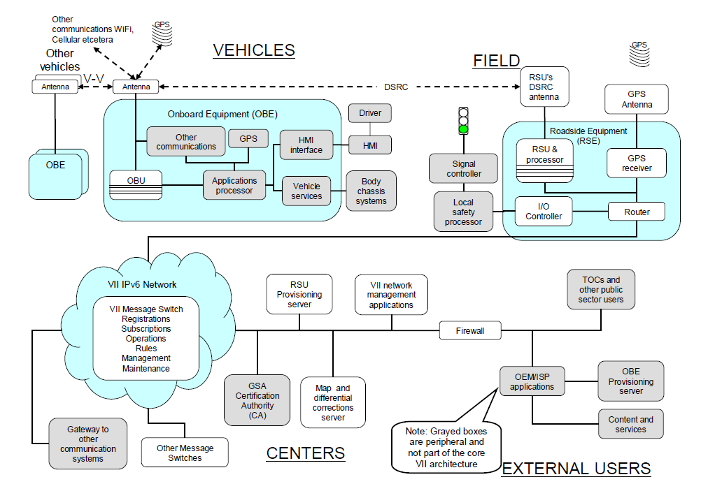
A typical V2I architecture can be seen in Figure 134 which was defined in Vehicle Infrastructure Integration program of USDOTs’ ITS Joint Program Office.
9.2. Wireless Technologies
9.2.1. DSRC
For V2I applications the same communication standards are used as in V2V systems. The standards mentioned in Section 8.2 take into consideration the infrastructure and its requirements. In the architecture definitions the concept of the RSU has been elaborated.
9.2.2. Bluetooth
Bluetooth technology is a wireless communications technology that is simple, secure, and can be found almost everywhere. You can find it in billions of devices ranging from mobile phones and computers to medical devices and home entertainment products. It is intended to replace the cables connecting devices, while maintaining high levels of security. Automotive applications of Bluetooth technology began with implementing the Hands Free Profile for mobile phones in cars. The development is coordinated by the Car Working Group (CWG) and is ongoing ever since 2000 by implementing different profiles and new features. The key features of Bluetooth technology are ubiquitousness, low power, and low cost. The Bluetooth Specification defines a uniform structure for a wide range of devices to connect and communicate with each other.
When two Bluetooth enabled devices connect to each other, is the so-called pairing. The structure and the global acceptance of Bluetooth technology means any Bluetooth enabled device, almost everywhere in the world, can connect to other Bluetooth enabled devices located in proximity to one another.
Connections between Bluetooth enabled electronic devices allow these devices to communicate wirelessly through short-range, creating ad hoc networks commonly known as piconets. Piconets are established dynamically and automatically as Bluetooth enabled devices enter and leave radio proximity meaning that you can easily connect whenever and wherever it's convenient for you. Each device in a piconet can also simultaneously communicate with up to seven other devices within that single piconet and each device can also belong to several piconets simultaneously. This means the ways in which you can connect your Bluetooth devices is almost limitless. There are applications that even do not require a connection establishment. It may be enough if the Bluetooth device’s wireless option is set to “visible” and “shown to all”, because fixed positioned Bluetooth access points may detect the movement of the Bluetooth device from one AP to another AP. This technology can easily be used for measuring the traffic flow.
A fundamental strength of Bluetooth wireless technology is the ability to simultaneously handle data and voice transmissions, which provides users with a variety of innovative solutions such as hands-free sets for voice calls, printing and fax capabilities, and synchronization for PCs and mobile phones, just to name a few.
The range of Bluetooth technology is application specific. The Core Specification mandates a minimum range of 10 meters or 30 feet, but there is no set limit and manufacturers can tune their implementations to provide the range needed to support the use cases for their solutions.
Range may vary depending on class of radio used in an implementation:
Class 3 radios – have a range of up to 1 meter or 3 feet
Class 2 radios – most commonly found in mobile devices – have a range of 10 meters or 33 feet
Class 1 radios – used primarily in industrial use cases – have a range of 100 meters or 300 feet
Bluetooth technology operates in the open and unlicensed industrial, scientific and medical (ISM) band at 2.4 to 2.485 GHz, using a spread spectrum, frequency hopping, full-duplex signal at a nominal rate of 1600 hops/sec. The 2.4 GHz ISM band is available and unlicensed in most countries. The most commonly used radio is Class 2 and uses 2.5 mW of power. Bluetooth technology is designed to have very low power consumption. This is reinforced in the specification by allowing radios to be powered down when inactive.
Bluetooth technology's adaptive frequency hopping (AFH) capability was designed to reduce interference between wireless technologies (such as WLAN) sharing the 2.4 GHz spectrum. AFH works within the spectrum to take advantage of the available frequency. This is done by the technology detecting other devices in the spectrum and avoiding the frequencies they are using. This adaptive hopping among 79 frequencies at 1 MHz intervals gives a high degree of interference immunity and also allows for more efficient transmission within the spectrum. For users of Bluetooth technology this hopping provides greater performance even when other technologies are being used along with Bluetooth technology. The AFH technology is shown in Figure 135 [118].
The newest Bluetooth Technology is Bluetooth 4.0 called Bluetooth Smart (Low Energy) Technology. While the power-efficiency of Bluetooth Smart makes it perfect for devices needing to run off a tiny battery for long periods, the most important attribute of Bluetooth Smart is its ability to work with an application on the smartphone or tablet you already own. Bluetooth Smart wireless technology features:
Ultra-low peak, average and idle mode power consumption
Ability to run for years on standard coin-cell batteries
Low cost
Multi-vendor interoperability
Enhanced range
In automotive industry the primary usage of Bluetooth connects hands-free car systems which help drivers focus on the road. Another special usage is health monitoring e.g. people with diabetes can monitor their blood-glucose levels by using a Bluetooth glucose-monitoring device paired with the car. Also in-vehicle intelligent interfaces may provide e.g. vehicle related technical information to the driver via a Bluetooth channel. (Source: [119])
In V2I systems Bluetooth can be used to provide communication channel between the car and the traffic signal systems. Nowadays several manufacturers offer Bluetooth capable traffic control devices. It is capable for privileging the public transport at the intersections or measuring the traffic and pedestrian flows with the help of the electronic devices installed with Bluetooth radio (such as smartphones, tablets, navigation units etc.). These systems detect anonymous Bluetooth signals transmitted by visible Bluetooth devices located inside vehicles and carried by pedestrians. This data is then used to calculate traffic journey times and movements. It reads the unique MAC address of Bluetooth devices that are passing the system. By matching the MAC addresses of Bluetooth devices at two different locations, not only the accurate journey time is measured, privacy concerns typically associated with probe systems are minimized.
9.2.3. WiFi
WiFi (Wireless Fidelity) or WLAN (Wireless Local Network) communication system is based on the Institute of Electrical and Electronics Engineers' (IEEE) 802.11 standards. The 802.11 family consists of a series of half-duplex over-the-air modulation techniques that use the same basic protocol. The most popular are those defined by the 802.11b and 802.11g protocols, which are amendments to the original standard. 802.11-1997 was the first wireless networking standard in the family, but 802.11b was the first widely accepted one, followed by 802.11a, 802.11g and a multi-streaming modulation 802.11n. Other standards in the family (c–f, h, j) are service amendments and extensions or corrections to the previous specifications. The IEEE 802.11p WAVE is intended to amend the overall IEEE 802.11 standard as mentioned in Section IEEE 802.11p (WAVE) 8.2.1.
802.11b and 802.11g use the 2.4 GHz ISM band. Because of this choice of frequency band, 802.11b and equipment may occasionally suffer interference from microwave ovens, cordless telephones and Bluetooth devices. 802.11b and 802.11g control their interference and susceptibility to interference by using direct-sequence spread spectrum (DSSS) and orthogonal frequency-division multiplexing (OFDM) signalling methods, respectively.
The “general” IEEE 802.11 standards (that used in consumer electronics) can support only infotainment applications in the vehicle. Only the IEEE 802.11p WAVE (DSRC) is capable for safe and reliable communications in V2X applications.
9.2.4. Mobile networks
The most wide-spread mobile (cellular) network technology is GSM (Global System for Mobile communication). GSM was designed principally for voice telephony, but a range of bearer services was defined (a subset of those available for fixed line Integrated Services Digital Networks, ISDN), allowing circuit-switched data connections at up to 9600 bits/s. The technology behind the Global System for Mobile communication (GSMTM) uses Gaussian Minimum Shift Keying (GMSK) modulation, a variant of Phase Shift Keying (PSK) with Time Division Multiple Access (TDMA) signalling over Frequency Division Duplex (FDD) carriers. Although originally designed for operation in the 900 MHz band, it was soon adapted also for 1800 MHz. The introduction of GSM into North America meant further adaptation to the 800 and 1900 MHz bands. Over the years, the versatility of GSM has resulted in the specifications being adapted to many more frequency bands to meet niche markets.
At the time of the original system design, this rate compared favourably to those available over fixed connections. However, with the passage of time, fixed connection data rates increased dramatically. The GSM channel structure and modulation technique did not permit faster rates, and thus the High Speed Circuit-Switched Data (HSCSD) service was introduced in the GSM Phase 2+.
During the next few years, the General Packet Radio Service (GPRS) was developed to allow aggregation of several carriers for higher speed, packet-switched applications such as always-on internet access. The first commercial GPRS offerings were introduced in the early 2000s. Meanwhile, investigations had been continuing with a view to increasing the intrinsic bit rate of the GSM technology via novel modulation techniques. This resulted in Enhanced Data-rates for Global Evolution (EDGE), which offers an almost three-fold data rate increase in the same bandwidth. The combination of GPRS and EDGE brings system capabilities into the range covered by the International Telecommunication Unions IMT-2000 (third generation) concept, and some manufacturers and network operators consider the EDGE networks to offer third generation services.
In 1998, the ETSI (European Telecommunications Standards Institute) General Assembly took the decision on the radio access technology for the third generation cellular technology: wideband code-division multiple access, W-CDMA, would be employed. A dramatic innovation was attempted: a partnership project was formed with other interested regional standards bodies, allowing a common system to be developed for Europe, Asia and North America. The Third Generation Partnership Project (3GPP) was born. (Source: [120])
The Third Generation mobile cellular technology developed by 3GPP - known variously as Universal Mobile Telecommunications System (UMTS), Freedom of Mobile Multimedia Access (FOMA), 3GSM, etc., is based on wideband code division multiple access (W-CDMA) radio technology offering greater spectral efficiency and higher bandwidth than GSM. UMTS was originally specified for operation in several bands in the 2 GHz range. Subsequently, UMTS has been extended to operate in a number of other bands, including those originally reserved for Second Generation (2G) services. The UMTS radio technology is direct-sequence CDMA, each 10 ms radio frame is divided into 15 slots.
As a development of the original radio scheme, a high-speed download packet access (HSDPA, offering download speeds potentially in excess of 10 Mbit/s), and an uplink equivalent (HSUPA, also sometimes referred to as EDCH) were developed. Collectively the pair are tagged HSPA, and permit the reception of multimedia broadcast/multicast, interactive gaming and business applications, and large file download challenging traditional terrestrial or satellite digital broadcast services and fixed-line broadband internet access. The radio frames are divided into 2 ms subframes of 3 slots, and gross channel transmission rates are around 14 Mbit/s.
3GPP's radio access undergoes continuous development and the 'long-term evolution' (LTE) exercise aims to extend the radio technology to keep UMTS highly competitive to potential rival technologies, with data rates approaching 100 Mbit/s by the end of the decade. (Source: [121])
9.2.5. Short range radio
Short range radio means an older technology, which is wide-spread in case of public transport vehicles. They have been installed with a short range radio transmitter which works on a lower ISM band (such as 433 or 868 MHz). It can broadcast an identifier which can be received by the traffic control systems’ roadside beacon and thus the public transport vehicles can be prioritized in the intersections or by the stops.
9.3. Applications
As mentioned above the V2I systems are closely related to the V2V communications. Most of the V2I applications rely on the V2V on-board units, so these applications can commonly called Intelligent Transportation System (ITS) applications. Naturally several applications currently exist which based only on roadside sensors, typically which require only observation (e.g. toll control, speed measurement etc.).
9.3.1. Safety
The safety applications aim to decrease the number of accident by prediction and notifying the drivers of the information obtained through the communications between the vehicles and sensors installed on the road.
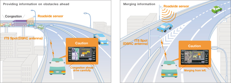
The typical safety applications could be the following:
warning for hazardous situations (such as congestions, accidents, obstacles etc.),
merging assistance,
intersection safety,
speed management,
rail crossing operations,
priority assignment for emergency vehicles.
9.3.2. Efficiency
The efficiency applications can support the better utilization of the roads and intersections. These functions can operate locally at an intersections or a given road section, or in an optimal case on a large network, such as a busy downtown. It is important to note that the efficiency applications also have a beneficial effect on safety in most cases.
The following typical applications can enhance the traffic efficiency:
traffic jam notification,
prior recognition of potential traffic jams,
dynamic traffic light control,
dynamic traffic control,
connected navigation
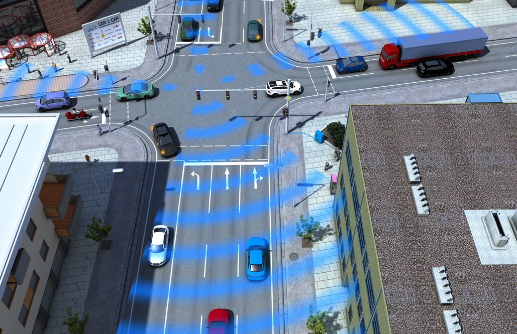
9.3.3. Payment and information
The number plate recognition serves as base for the payment applications, which is well-tried and reliable camera-based technology. The payment applications could be the following:
parking control,
congestion charge,
highway toll control.
The information services can be typically the conventional variable traffic signs or temporary road signs supplemented with a DSRC beacon.
Chapter 10. Vehicle to Environment interactions (V2E)
Not only the highly automated vehicles with intelligent sensors can position the vehicle in the surrounding environment, but the environment can also sense and position the vehicle with intelligent infrastructure.
These technologies can support (even with the help of V2V and V2I) vehicle detection and movement measurement, furthermore the detection of pedestrians and cyclists and essential for the Intelligent Transportation Systems (ITS).
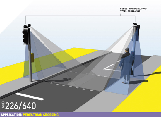
The following subsections will introduce the elements of this intelligent infrastructure.
10.1. Conventional technologies
Conventional (often called "in-situ") technologies refer to traffic data measured by the means of detectors located along the roadside. A short overview is presented in the following chapters based on [122]. Generally, traffic count technologies can be split into two categories: the intrusive and non-intrusive methods. The intrusive methods basically consist of a data recorder and a sensor placing on or in the road. They have been utilized for many years and the most important ones are briefly described hereafter.
Pneumatic road tubes: rubber tubes are placed across the road lanes to detect vehicles from pressure changes that are produced when a vehicle tire passes over the tube. The pulse of air that is created is recorded and processed by a counter located on the side of the road. The main drawback of this technology is that it has limited lane coverage and its efficiency is subject to weather, temperature and traffic conditions. This system may also not be efficient in measuring low speed flows.
Piezoelectric sensors: the sensors are placed in a groove along roadway surface of the lane(s) monitored. The principle is to convert mechanical energy into electrical energy. Indeed, mechanical deformation of the piezoelectric material modifies the surface charge density of the material so that a potential difference appears between the electrodes. The amplitude and frequency of the signal is directly proportional to the degree of deformation. This system can be used to measure weight and speed.
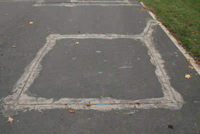
Magnetic loops: it is the most conventional technology used to collect traffic data. The loops are embedded in roadways in a square formation. The detector powers the loop that generates a magnetic field. The loop resonates at a constant frequency that the detector monitors. When a large metal object, such as a vehicle, moves over the loop, the resonance frequency changes, thus the vehicle passing by can be detected. The information is then transmitted to a counting device placed on the side of the road. This has a generally short life expectancy because it can be damaged by heavy vehicles, but is not affected by bad weather conditions. This technology has been widely deployed in Europe (and elsewhere) over the last decades. However, the implementation and maintenance costs can be expensive.
A non-intrusive solution is the passive magnetic sensors, which are fixed under or on top of the roadbed. They count the number of vehicles, their type and speed. However, in operating conditions the sensors have difficulties in differentiating between closely spaced vehicles.
10.2. Camera-based systems
For camera technologies please refer to the Section 3.3. Here some specialties and applications are introduced.
Passive and active infra-red: the presence, speed and type of vehicles are detected based on the infrared energy radiating from the detection area. The main drawbacks are the performance during bad weather, and limited lane coverage.
Video image detection is also used in traffic flow measurement: video cameras record vehicle numbers, type and speed by means of different video techniques e.g. trip line and tracking.
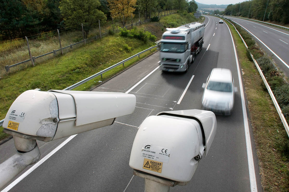
Video image detection can also be used for functions based on vehicle identification like parking garage control, highway toll collect control, or average speed detection. Long term average speed detection is based on the identification (number plate) of the vehicle at different fixed points of the infrastructure (e.g. highway). As the distance between the fixed measuring points are known the average vehicle speed can be calculated from the time of appearance. The system can be sensitive to meteorological conditions.
10.3. Radar, ultrasonic and laser detectors
For radar, laser and ultrasonic technologies please refer to the Section 3. Here some specialties and applications are introduced.
Microwave radar: this technology can detect moving vehicles and speed (Doppler radar). It records count data, speed and simple vehicle classification and is not affected by weather conditions. Not only the police use fixed or portable radar (LIDAR) systems for speed control of the vehicles, but local communities are operating the same technology for setting up fixed speed warning signs at the entrance of the city (village) or just before a dangerous curve.
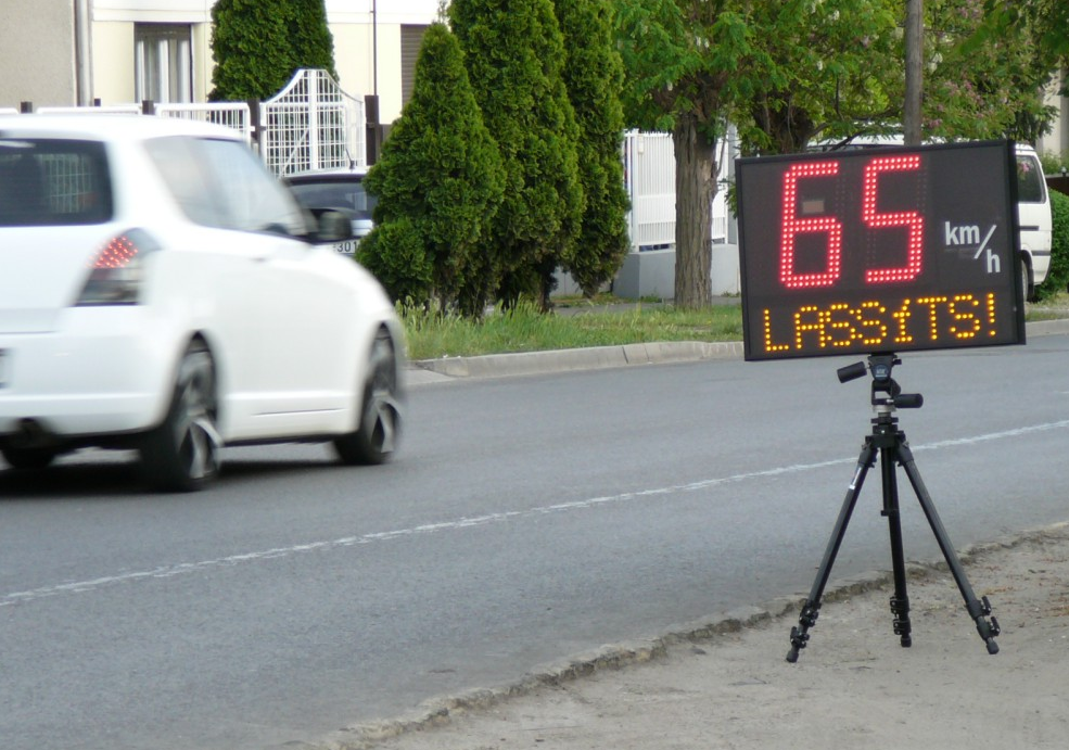
Ultrasonic and passive acoustic: these devices emit sound waves to detect vehicles by measuring the time for the signal to return to the device. The ultrasonic sensors are placed over the lane and can be affected by temperature or bad weather. The passive acoustic devices are placed alongside the road and can collect vehicle counts, speed and classification data. They can also be affected by bad weather conditions (e.g. low temperatures, snow).
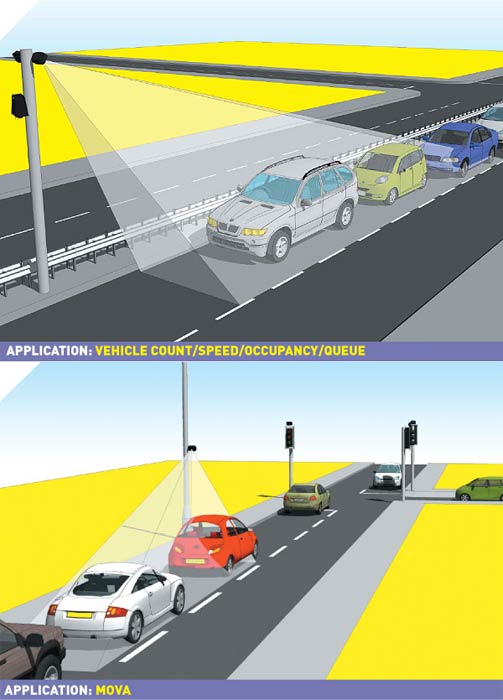
10.4. Floating Car Data (FCD)
The principle of FCD is to collect real-time traffic data by locating the vehicle via mobile phones or GPS over the entire road network. This basically means that every vehicle is equipped with mobile phone or GPS which acts as a sensor for the road network. Data, such as car location, speed and direction of travel are sent anonymously to a central processing centre. After being collected and extracted, useful information (e.g. status of traffic, alternative routes) can be redistributed location based to the drivers on the road. FCD is an alternative or rather complement source of high quality data to existing technologies. They will help improve safety, efficiency and reliability of the transportation system. They are becoming crucial in the development of new Intelligent Transportation Systems (ITS). (Source: [122])
Chapter 11. Different methods for platooning control
The number of persons and volume of goods transported on the roads have increased significantly. Simultaneously, requirements have also increased. Here are some examples: a need to enhance passenger comfort, to improve road holding, the efficiency of transport, the safety of travel, the reliability of vehicle components and also to reduce fuel consumption and the time transport takes, etc. The vehicle industry primarily focuses on the re-design of vehicle components or the efficiency of different vehicle functions. In this sense the application of active components with high versatility has great potential.
Another direction addresses the joint control of vehicle groups. The term platoon is used to describe several vehicles operated under automatic control as a unit when they are traveling at the same speed with relatively small inter-vehicle spacings. According to the principle of the platoon, the first vehicle is driven by a professional driver, while the following vehicles are under automated longitudinal and lateral control and these drivers are able to undertake other tasks. The following vehicle driver must be able to take over control of the vehicle in the event of a controlled or unforeseen dissolving of the platoon. A well-organized platoon control may have advantages in terms of increasing highway capacity and decreasing fuel consumption and emissions.
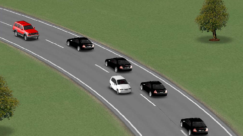
The thoughts of platoon control were motivated by intelligent highway systems and road infrastructure, see the PATH program in California and the MOC-ITS program in Japan. The European programmes were based on the existing road networks and infrastructure and focused mainly on commercial vehicles with their existing sensors and actuators, see [123], [124], [125]. The main goal of the projects was to examine the operation of platoons on public motorways with full interaction with other vehicles. In a Hungarian project an automated vehicle platoon of heavy vehicles was developed. The goal of the project was to analyze the control algorithms and synthesize the experimental results, see [126].
The control design is based on external factors such as traffic situations (traffic jam), terrain characteristics (straight, road slopes), road types (highway, secondary road), speed limits. It is also based on different internal factors such as the dynamic abilities of vehicles in the platoon, their emission properties, reliability. Since the safe and economical motion of the platoon is determined by the leader vehicle, it is crucial for the leader vehicle to use this piece of information during the journey. The schematic structure of the controlled platoon system is shown in Figure 144.
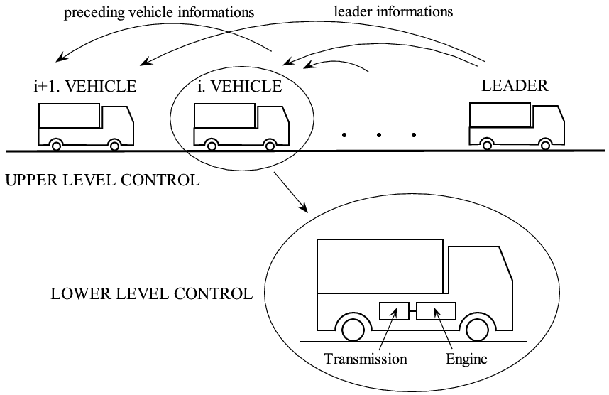
11.1. Control tasks
The vehicle following control law is said to provide individual vehicle stability if the spacing error of the vehicles converges to zero when the preceding vehicle is operating at constant speed. If the preceding vehicle is accelerating or decelerating, then the spacing error is expected to be nonzero. Spacing error in this definition refers to the difference between the actual spacing from the preceding vehicle and the desired inter-vehicle spacing.
Let  be the location of the
  vehicle measured from an inertial reference, see Figure 145.
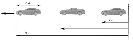
The spacing error for the  vehicle is then defined as
| (1) |
where  is the desired spacing and includes the preceding vehicle length. The desired spacing
  must be chosen as a function of variables such as the vehicle speed
  . The control law is said to provide individual vehicle stability if the following condition is satisfied
| (2) |
If the vehicle following control law ensures individual vehicle stability, the spacing error should converge to zero when the preceding vehicle moves at constant speed. However, the spacing error is expected to be non-zero during acceleration or deceleration of the preceding vehicle. It is important then to describe how the spacing error would propagate from vehicle to vehicle in a string of ACC vehicles that use the same spacing policy and control law.
The string stability of a string of ACC vehicles refers to a property in which spacing errors are guaranteed not to amplify as they propagate towards the tail of the string, see (1), (2). For example, string stability ensures that any errors in spacing between the  and
and cars does not amplify into an extremely large spacing error between cars
  and
and  when (
 ) further up in the string of vehicles.
In order to evaluate autonomous platoons from control point of view string stability and performance are analyzed. By definition, the platoon is string stable if, for a given  , there exist
  such that
| (3) |
where  and
and  . In other words the spacing errors remain bounded along the platoon whenever the initial spacing errors are bounded. It follows from the definition that the spacing errors due to changes in lead vehicle speed do not amplify along the platoon and in time when string stability is satisfied [127].
The following condition will be used to determine if the system is string stable:
| (4) |

where  is the transfer function relating the spacing errors of consecutive vehicles
  .
.
Platoon performance is commonly defined as either the largest peak spacing error or the total length of the platoon. In the paper, series
| (5) |
are evaluated from which both quantities can be derived. The infinity norm of a scalar signal  is defined by
  . From series
  ,
,  one can chose constant safety gaps
  and inspect the ability of the platoon to attenuate errors. Furthermore, the possibility of actuator saturation can be concluded.
Remark 1.1 It can be shown that an autonomous controller cannot ensure string stability when the constant spacing policy is used. In the constant spacing policy, the desired spacing between successive vehicles is defined by  where
where  is a constant and includes the length
  of the preceding vehicle. The spacing error of the i th vehicle is defined as
  . When the acceleration of the vehicle can be instantaneously controlled, then a linear control system of the type
  yields
  , which leads to the following closed-loop error dynamics
  . This equation shows the the propagation of spacing errors in the platoon of vehicles. The magnitude of the transfer function between
  and
and  may be greater than 1 so the autonomous control law is not string stable. Thus, in the case of the constant spacing policy, string stability cannot be ensured by autonomous control.
11.2. Platooning strategies
Two type os control strategies have been proposed:
Constant Spacing control strategies
Variable Spacing control strategies
In the Constant Spacing control strategies, the desired inter-vehicule spacing is independent of the velocity of the controlled vehicle. The tracking requirement is stringent, since every controlled vehicle has to match its position, velocity and acceleration with the vehicle ahead. As a consequence, these strategies require more information to guarantee performance. The achievable traffic capacity is very high in a constant spacing control strategy. There are several solutions for constant spacing strategy:
Control with information of reference vehicle information only
Control with information of preceding vehicle
Control with information of lead and preceding vehicles
Mini platoon control
In the Variable Spacing control strategies the desired inter-vehicle spacing varies with the velocity of the controlled vehicle. The tracking requirement is not as stringent as the previous case. Some of the variable spacing control strategies can be implemented with on-board sensors. A possible solution for variable spacing strategy is the
Autonomous
Intelligent Cruise Control.
In the following the main features of the most important three strategies are presented.
Case 1.1 Control with information of lead vehicle
The first method is based on the reference velocity information. Consider the following control law:
| (6) |
where  is the position of the lead vehicle in the platoon.
The spacing error dynamics is obtained using the following equation:  thus
thus  . This is the best achievable platoon performance. It is unsafe since it does not take the information of the preceding vehicle into consideration.
Case 1.2 Control with information of preceding vehicle
In this strategy control law is based only on the on-board sensor measurements. The control law is the following
| (7) |
and the spacing Error Dynamics is as follows:  thus
thus
| (8) |
for i=1  , where
  is the acceleration of the leader. The frequency function:
| (9) |
thus in the frequency domain
| (10) |
Since  , the spacing amplifying along the platoon. Consequently, the string stability is not fulfilled.
Case 1.3 Control with information of lead and preceding vehicles
The control strategy is based on lead vehicle acceleration, velocity and position information:
(11)
The string stability is guaranteed. The platoon control can be distributed into two control tasks: longitudinal control for speed tracking and lateral control for trajectory tracking.
In the simulation example four vehicles are traveling along an undulating road and the controller changes the reference velocities, which are tracked by the vehicles accurately, see Figure 3(a). The control signals are the longitudinal control forces, see Figure 3(d), which are realized by the throttle positions and the brake pressures.
|
|
|
|
|
|
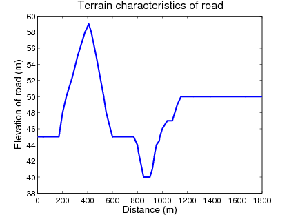
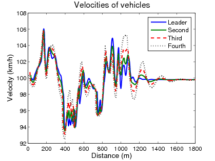
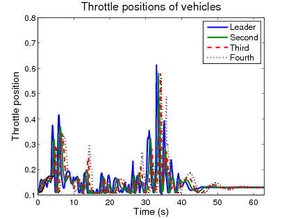
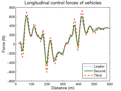
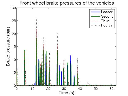
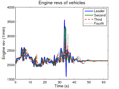
Figure 146: Simulation example
Remark 1.2 In the travelling the safety operation must be guaranteed. In the following three possible solutions for collision avoidance are presented.
Avoiding collision by grading vehicles: A possible way to handle saturation is to grade vehicles in the platoon in order of their dynamical ability.
Avoiding collision by modifying the velocity of the leader vehicle: In the strategy the communication with the leader vehicle is bidirectional. To avoid the saturation and the consequent split off of the following vehicles the velocity of the leader vehicle is moderated.
Avoiding collision by splitting platoon: In this lay-out the platoon dissolves into several platoons following each other, where the last vehicle of the preceding platoon serves as the reference vehicle for the following platoon.
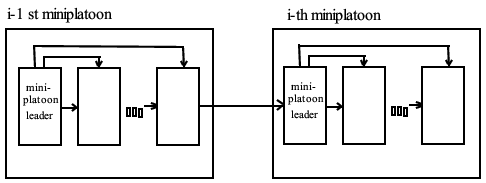
In another example the platoon is organized with dynamically different vehicles. The leader vehicle followed the target velocity adjusted by the onboard cruise control while saturation occurred in one of the the following vehicles. Vehicles in the platoon having worse mass/performance figures are not able to match the acceleration prescribed by their controller during uphill or heavy acceleration therefore they cannot keep the desired spacing.
Because of the splitting off the following vehicle prescribes bigger acceleration than necessary (due to the growing distance from the leader vehicle), hence the following vehicle can interfere with the saturating vehicle. Figure 6 shows that because if it is notable mass, the desired force related to the prescribed acceleration is too big. Hence saturation occurs at this vehicle, consequently it cannot match the prescribed acceleration and in this manner it splits off from the platoon. The significantly big spacing error with a negative sign shows the split off. Due to this, the fifth vehicle prescribes bigger acceleration than it is necessary, hence it runs into the fourth vehicle.
|
|
|
|
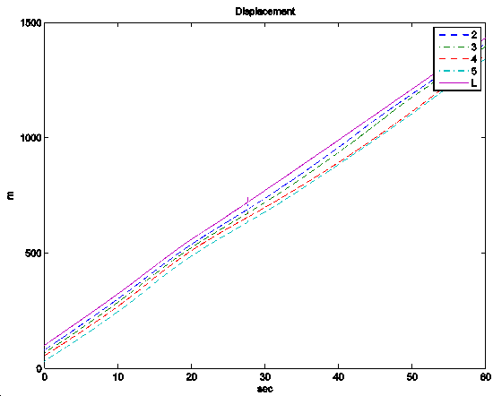
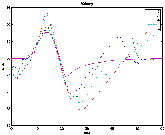
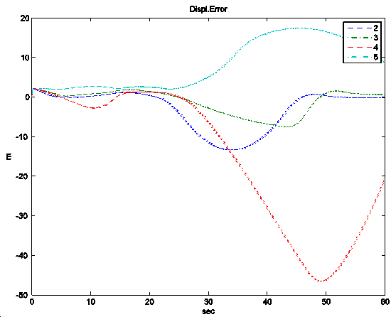
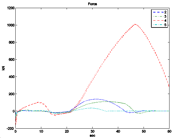
Figure 148: Simulation results with diverse vehicles
Chapter 12. Vehicle control considering road conditions
Two types of road disturbances are distinguished: stochastic (random) irregularities and deterministic disturbances.
Random road unevenness is characterized by its stochastic properties and can be regarded as disturbances of long or infinite duration. Deterministic road disturbance is mostly related to an excitation of short duration such as kerbs, speed humps and potholes. An accurate representation of the stochastic road irregularities is required in order to predict vehicle responses to road excitations, see [128], [129].
The stochastic description of road surfaces is useful for calculating average performance parameters, but such calculations do not account for the deterministic effect of road damage, obstacles and potholes, or for the high degree of regularity in road profiles that occasionally are present due to terrain features, road building practices or repeated traversal by vehicles.
A very simple model for the vertical road is a colored noise resulting from the application of a first-order shaping filter to a white noise signal. This process is given by the following differential equation:
| (12) |

where  is the road displacements at the respective springs,
  is a coefficient depending on the shape of the road irregularities and
  is the forward vehicle speed. The parameter
  needed for the considered road description is selected as follows:
  in asphalt,
  in concrete and
  in rough.
In order to classify different roads Hac has proposed a parameter based method, where the road signal was given by the following continuous time model, see [130]:
| (13) |
where  is a white noise process, parameters
  ,
, ,
, ,
, ,
, ,
, depend of the forward velocity and the road type. The calculation of the parameters are the following:

,  ,
,  ,
,
,  ,
,
,
,  ,
,  .
.
The relation between the characteristics that describe the road quality and the parameters defining the road model are given in Table 3.
Road Type |
|
|
|
|
|
asphalt | 0.2 | 0.05 | 0.6 | 7.65 | 1.36 |
paved | 0.5 | 0.2 | 2.0 | 2.55 | 4.5 |
dirt | 0.8 | 0.5 | 1.1 | 7.5 | 2.5 |


Using the measured data the effects of the forward velocity to the suspension system is illustrated in Figure 149. The effects of the road roughness to the suspension system when the velocity of the vehicle is  are shown in Figure 150.
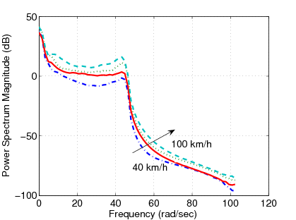
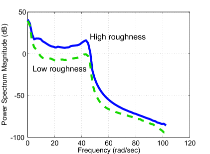
Chapter 13. Design of decentralized supervisory control
In a centralized control structure the main objective consist in a single main controller that send the control signals directly to the subsystems actuators. This kind of information flow increases the computational load in the central ECU requiring more powerful units. In the other hand the centralized structures are rigid, which limited its reconfiguration capabilities for integrating new elements in the control loop, so that if it is a need of integrating a new subsystem to the control loop the only solution is to redesign the complete control system. Also this type of topology forces the OEM’s to open its system architecture to its suppliers.
An integrated control system is designed in such a way that the effects of a control system on other vehicle functions are taken into consideration in the design process by selecting the various performance specifications. Redundancy on sensor and actuator levels makes it possible to realize the same functionality using different sensor and actuator configurations. Thus integrated design is also motivated by the needs of reconfigurable and reliable control, [131], [132].
A possible solution to an integrated control could be to set the design problem for the whole vehicle and include all the performance demands in a single specification. Besides the complexity of the resulting problem the formulation of a suitable performance specification is the main obstacle for this direct global approach. In the framework of available design techniques the formulation and successful solution of complex multi-objective control tasks are highly nontrivial, see e.g. [133], [134].
In a decentralized control structure every subsystem has its own independent controller and control objective which commands its particular actuator. The interaction among different control loops is limited to shared information obtained from a communication bus. This type of control structure was used in the early chassis control integration. In this scheme the integration lies on the OEM’s, while the supplier provides its systems interconnection options.
Another solution to the integrated control is a decentralized control structure where the components are designed independently, see e.g. [135], [136]. In the paper the decentralized control system is augmented with a supervisor as illustrated in Figure 151. The role of the supervisor is to meet performance specifications and prevent the interference and conflict between components. The supervisor has information about the current operational mode of the vehicle, i.e., the various vehicle maneuvers or the different fault operations. The supervisor is able to make decisions about the necessary interventions into the vehicle components and guarantee the reconfigurable and fault-tolerant operation of the vehicle. These decisions are propagated to the lower layers through predefined interfaces encoded as suitable scheduling signals.
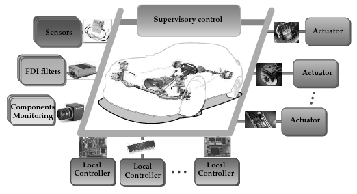
The role of the supervisor is to coordinate the local components and handle the interactions between them. Since the performance specifications of local controllers are often in conflict, the supervisor must also guarantee a balance or trade-off between them. The information provided by the supervisor is composed of messages and signals sent by the monitoring components and fault detection and isolation (FDI) filters. Based on this information the supervisor is able to make decisions about the necessary vehicle maneuvers and guarantee reconfigurable and fault-tolerant operation of the vehicle and send messages to the local controllers. In order to implement a safety feature the operation of a local controller must be modified by a supervisory command. This is realized through appropriately set scheduling variables that are transmitted to the local controllers. At a local level the behaviour of the controller is affected by these scheduling variables through the performance weighting functions. The difficulty in the supervisory control is that global stability and performance are difficult to guarantee.
The design of the supervisor does not involve dynamical systems explicitly. However, due to the time variation of the signals the designer should check the validity of relations between the momentary values of the monitoring signals based on a temporal logic. The difficult part of the design is to ensure the correctness of the specification. It must be stressed at this point that the baseline configurations handle only one actuator, which is associated with a given task (functionality). The hierarchy of the configurations and corresponding scheduling variables ensure that the additional actuator(s) considered improve the stability properties of the given functionality.
In contrast to the controller switching strategy the proposed approach uses a performance weighting strategy. On the supervisor level the required configurations are defined uniquely by the specific values of a set of marker signals. These marker signals are used as scheduling variables on the level of local controllers. The task of the supervisor design is to specify these marker signals in such a way that the different combinations of their values define the specific event (functionality) in a unique way. The different combinations of the marker signals encode the designers specification (option) in dealing with multi-objective or conflicting scenarios.
A local component is a well-defined ensemble of a controller, an actuator and a set of related physical or virtual sensors, e.g., units for monitoring components and FDI filters. These elements are able to detect emergency vehicle operations, various fault operations or performance degradations in controllers. They send messages to the supervisor in order to guarantee the safe operation of the vehicle.
Each of the local components is governed by a local controller. A local controller must meet the predefined performance specifications. The signals of monitoring components and those of FDI filters are built in the performance specifications of the controller by using a parameter-dependent form. The performance specifications are formalized in a parameter-dependent way in which the corresponding scheduling variable is given by the supervisor. Thus the controller is able to modify or reconfigure its normal operations in order to focus on other performances instead of the actual performances. It sends messages about the changes to the supervisor and it receives messages from the supervisor about the special requirements.
The efficient operation of the supervisor and the local controllers require reliable and highly accurate signals from the system. To meet this requirement redundant sensors, diverse calculations and fault detection filters are needed. To achieve the efficient and optimal intervention the detections of faulty sensors are important since they must be substituted for in operations based on these sensors. Low cost solutions are preferred in the vehicle industry, thus simple sensors and software-based redundancy must be applied.
In the following two examples for monitored components related to specific control goals are presented:
Yaw stability is achieved by limiting the effects of the lateral load transfers. The purpose of the control design is to minimize the lateral acceleration, which is monitored by a performance signal. Unilateral braking is one of the solutions, in which brake forces are generated in order to achieve a stabilizing yaw moment. In the second solution additional steering angle is generated in order to reduce the effect of the lateral loads. These solutions, however, require active driver intervention into the motion of the vehicle to keep the vehicle on the road.
Roll stability is achieved by limiting the lateral load transfers on both axles to below the levels for wheel lift-off during various vehicle maneuvers. The aim of the control design is to reduce the maximum value of the lateral load transfer if it exceeds a predefined critical value.
Chapter 14. Fleet Management Systems
The Fleet Management System collects, store and provide complete comprehensive information about the current state of the vehicles and cargo, the route history, the expected events, as well as the driver activities for the vehicle maintenance and operator companies.
The main fields of application are the following:
vehicle operation,
traffic safety,
security of freight,
traffic management,
environmental protection.
14.1. Motivation
Thanks to the rapid development of microelectronics and mobile telecommunications by the end of the 90’s a wider range of fleet diagnostics and satellite tracking became possible. These innovations gave a technological background of the creation of fleet management systems. Economical demand for Fleet Management Systems strengthened as an effect of the increased competitive situation in passenger and freight transport especially in road traffic. This effect was strengthened by the growth of traffic density and the intensification of transportation demand in Europe. One of the social impacts of this progression is an increase in the number of accidents that intensifies the demand for safer vehicles.
Spread in on-line Fleet Management Systems was greatly aided by the constant decrease of communication charges and the increase of speed in mobile data transmission.
For all these reasons in the 2000s on-line Fleet Management Systems spread rapidly.
Its’ advantages are the following:
a greater safety in delivery,
aiding dynamic freight arrangement,
constant tracking of the mechanical condition of the vehicles,
reduction of operational costs (fuel consumption and maintenance costs),
avoidance of the illegal usage of the vehicle and the fuel manipulation,
easier documentation (e.g. journey log),
driver motivating system (driving style analysis),
developing safety of traffic (speeding and accident detection),
developing security of freight,
increased environmental protection.
In the following sections the structure, the elements, the functions, and the operation of the Fleet Management System will be introduced, with a special regard on on-line systems.
14.2. General requirements in transportation
14.2.1. Cost reduction
The main reason of the installation of a Fleet Management System is the expected decrease in the overall operating costs of the company. Though the establishment of such a system requires one-time costs of investment and its operation also imply costs, but these expenses are counterbalanced by the savings. The cost reductions arising from the more effective operation are typically the followings:
Reduction of operation costs thanks to the increase in vehicle utilization and optimal route planning.
The Fleet Management System provides the possibility of the maximal utilization of the vehicle parts’ lifetime by the complex monitoring of the vehicle. Simultaneously it warns for the necessity of the replacement and supports the logistics solutions also.
The system may improve the quality of the estimation of the fuel norm through the measurement of the real consumption.
14.2.2. Logistics management
The possibility of on-line vehicle tracking is an ideal tool for the optimization of the logistic processes. Not only the route of the goods can be determined, but the vehicle movements can be optimized. The improvement in logistics costs could be the followings:
Improve efficiency of freight transport
Decrease of extra charges caused by the delays.
Significant decrease in vehicle stop time can be reachable resulting in cost reduction with keeping the same transportation performance.
Monitoring helps forcing back the illegal utilization of the company’s vehicle.
Another requirement is to provide the safety of the freight through using Fleet Management System. The data acquired make possible to follow or retrace the vehicle events. With using on-line system it is possible to intervene in critical situations and to monitor the keeping the traffic regulations.
The following section presents the kind of functionality and the system architecture that can satisfy the above mentioned requirements.
14.2.3. Vehicle categories
Initially the Fleet Management Systems were introduced by the international transport companies with heavy commercial vehicles (large goods vehicle). These early systems have collected only the GPS positions and sent it by SMS to the central server. With the reduction of costs the FMS solutions have broken into the segment of the smaller commercial vehicles (light commercial vehicles). Nowadays the FMS is used almost in all vehicle segments, typically in the following ones:
large goods vehicle (commercial vehicles over 3.5 tons)
light commercial vehicles (commercial vehicles not more than 3.5 tons)
passenger vehicles
construction and agricultural machinery
14.3. System Functions
Early FMS systems, Initially the FMS systems were only capable of identifying GPS position and sending it in an SMS to the central server. Over the past decade the Fleet Management Systems have gone through a tremendous development. Nowadays these systems use several sensor sources, on-line packet switched data connection, bidirectional communication, feedback, on-board vehicle communication buses, improved MMI and driver identification, digital tachograph data etc. In the following subsections the system function groups will be detailed.
14.3.1. Data acquisition
Data acquisition and data handling give the basis of Fleet Management Systems. Primarily the on-board system should register existing vehicle signals, still in several cases the system needs new or more detailed parameters. Several possibilities are available for measuring the physical parameters and acquiring identification data (driver, trailer etc.). Nowadays all commercial vehicles possess multiple CAN interfaces providing various signals.
14.3.2. Data processing
Data processing includes the sampling of various sensor sources either dynamically or fixed time based. Sampling strategy determines the overall amount of data to be handled, that may require temporary storage and pre-processing (e.g. histogram generation) to lower communication costs.
14.3.3. Data transmission
There are two categories of Fleet Management Systems, depending on the data location. If there is a recording unit in the vehicle and the recorded data are processed and evaluated afterwards, it is called off-line Fleet Management System. When all the vehicles are connected on-line to a computer server over mobile internet, and real-time information and data evaluation is available, is called the on-line Fleet Management System. In the recent years the on-line systems have come into general use as the result of the evolution of the wireless communication technologies. Several communication possibilities have become reachable for fleet management systems. The generally used techniques are based on GSM networks mainly on packet-switched services (like GPRS). In the future UMTS technologies will expand the possibilities and data bandwidth will be no longer a bottleneck for any function.
14.3.4. Identification tasks
The identification of the motor vehicle is an essential task in Fleet Management Systems. This function can be achieved in several ways. The general solution is to use the “natural” identifier of the GSM unit called IMEI number which can be connected to the vehicle’s license plate or the vehicle identity number (VIN) in the central server’s relational database.
Identification increases system safety by connecting the vehicle data to the driver. Driver identification is very important from several aspects: work time registration, responsibility issues in case of special events etc. Nowadays a lot of different solutions can be reached on the market such as proximity (RFID) cards, Dallas keys, but recently the smart card based digital tachographs opened new possibilities on this field.
Another highly important task is trailer identification which is necessary for cargo tracking. It can be realized via the spiral cable between the tractor and the trailer or with a wireless identification system.
14.3.5. Alerts
Event-triggered alerts enable the system to indicate abnormal operations to the driver and to the system centre also. These functions generally monitor specified signals. In case these signals reach unexpected or dangerous value an event will occur. For example these events can be the sudden decrease of the fuel level, speeding, tyre pressure etc.
Specific characteristic of the alerts is that they are real-time to enable quick intervention.
14.3.6. Positioning
Determining the vehicle’s location is usually performed by GNSS systems (see Section 3.8). The principles of the satellite-based navigation systems (called GPS) were developed in the United Sates for military navigation purposes. The GPS is a widespread and reachable positioning solution which is capable of determining 3D position, chronometry and measurement of velocity. The system uses satellite signals for the determination of the position, thus it ensures continuous measurement possibility in 0-24 hours on the whole World. The Fleet Management Systems usually use GPS receivers or combined GPS/GLONASS receivers.
14.3.7. Central system (Back office)
The central system of the fleet management systems is a complex hardware and software system, which handles data acquisition, storage and evaluation tasks. The incoming data from the vehicles must be handled in safe and reliable way for avoiding data loss and unauthorized access. The central system generates reports, charts, alerts and handles the geographic tasks.
14.3.8. User system (Front office)
Since the front office is the interface to the staff operating the system, it has to provide the following functionalities: primarily the system operator should gather vehicle, route and driver data through customizable reports. In addition for the tasks of on-line fleet control it has to possess geographical algorithms, and visualization. Since data security is highly important in such systems, the authentication and authorization in the whole system including the back office and also the front office must be managed and designed carefully.
14.4. Architecture of Fleet Management Systems
General construction of on-line fleet management systems are demonstrated on Figure 152. Usually it consists of three main sub-systems, see [137]:
on-board units,
central server,
user computers.
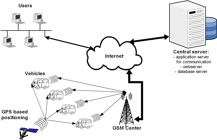
The operation of the system is the following. The on-board units (OBU) measure the operational parameters of the vehicle (state of the switches, energy consumption, motor parameters, etc.), and its position (aided by GPS-based location), and they store the data given by the driver (the name of the actual activity, etc.). These parameters are sent to a central server at the actualization of previously defined events (alarm-signal, sudden decrease in fuel level, etc.) and in previously defined periods of time.
On-board units communicate with the central server through mobile systems. The incoming data are evaluated and stored in a relational database. If necessary the central server can send an alarm to a given e-mail address or even a mobile phone. In this structure the communication from the server towards the vehicle is plausible as well. Aided by this the incoming data packages can be confirmed, a text message can be sent to the driver and the parameters of the on-board unit can be set.
Vehicles are detectable and observable almost constantly (on-line) and the operating parameters (running performance of vehicles, energy consumption, activities and work time of drivers, delivery performance) can be followed by a later evaluation of data stored in the centre (off-line).
14.4.1. On-board units (OBU)
In the building of the on-board unit (Figure 153) the important aspects are a heavy-duty design (EMC protection, shake protection, fluctuation of environmental temperature, etc.) and modularity. Therefore one should use a system that is built up of individual units. The connection of these by a series communication connection is worth realizing for the sake of simplicity and easy expansion.
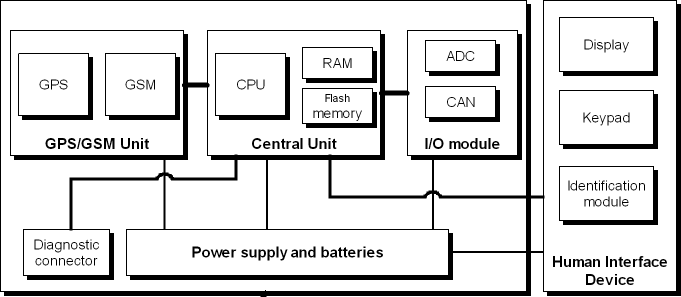
The on-board unit is made up of the following main units:
GSM/GPS module,
central unit,
human interface device,
diagnostic adapter,
I/O module,
power supply unit and background batteries.
The basic on-board units are often referred to as AVL. The abbreviation of AVL stands for Automatic Vehicle Locator[138], most commonly called as vehicle tracking device. There are GPS and/or GLONASS based positioning systems integrated together with an industrial GSM/UMTS modem, which sends the positioning information on-line to a central computer server. AVL devices may be extended with vehicle technical information like fuel tank level, engine revolution, fuel used, and so on.
14.4.1.1. In-Vehicle Data Acquisition
The most important and most complex function of the on-board unit is the exact acquisition of the vehicle data with special regard to the fuel consumption.
There are two ways to collect the necessary data:
sensor retrofit
in-vehicle communication buses
Formerly the first alternative was used generally because of the low penetration and hard reachability of the in-vehicle communication buses. This solution has several drawbacks, such as high cost, low reliability and accuracy, safety and warranty problems etc.
The other solution is generally based on the CAN bus technology, see [139]. CAN stands for Controller Area Network, meaning a computer network formulated by the vehicle’s electronic control units (ECU). CAN was primarily developed for automotive applications but later - due to its simplicity, reliability and electromagnetic immunity - it appeared also in industrial (CANopen), military (MilCAN), aerospace (CANaerospace) and nautical (SeaCAN) applications.
CAN bus is an asynchronous (time-shifted) serial bus system, originally developed by Robert Bosch GmbH from 1983 to interconnect electronic control units (ECU) in motor vehicles and was introduced in different steps to reduce cable harnesses and thereby weight. Instead of using an electrical circuit for each transmitted signal, the "bus" is based on a communication platform that regulates the relaying of messages between several devices.
In a practical context, the process is as follows: While the rear light was actuated by means of guiding a current to the rear light, the bus system only relays a message: "Light switch to rear light: Switch on!" Translating all control signals into messages requires a "greater intelligence" of the connected devices, at the same time this implies that many devices can exchange information, virtually at same time, using a very limited number of cable connections. (Source: [140])
All the necessary vehicle data is reachable on one of the vehicle CAN buses. There are great numbers of vehicle manufacturers having different types of vehicles on the market. They all have specific in-vehicle communication systems. To be able to “understand” each vehicle, one has to learn all these specific “languages”. Practically that means the developers of the Fleet Management Systems cannot interpret the data on the vehicle’s CAN bus. It is caused by the lack of the standardization of the CAN messages or the slight of the standards by the vehicle manufacturers.
In 2002, six major truck manufacturers (Volvo, Scania, Iveco, MAN, DAF, Mercedes-Benz) decided to create a standardized vehicle interface for these GPS based tracking systems, called the Fleet Management System Standard (FMS Standard). Since the establishment of the FMS Standard, there is no need to learn just one “language”. No matter which OEM produced a vehicle, if it was equipped with an FMS interface (FMS Gateway), there is the same output for all vehicles. The standard itself was a huge step forward in fleet management, since telematics devices (AVL) could access vehicle technical information without the need of vehicle specific developments.
FMS Standard versions:
FMS Standard 1.0 (Initial standard issued in 2002)
Bus FMS standard (Ver. 00.01 issued in 2007, specialized standard for buses and coaches including specific signals like door openings, etc. Since then the original “FMS Standard 1.0” was also referred as “Truck FMS Standard”)
FMS Standard 2.0 (extended standard issued in 2010. This standard took over some signals from the Bus FMS Standard, but FMS Standard 2.0 was still handled separately for Trucks.)
FMS Standard 3.0 harmonized Bus and Truck standard (issued in 2012). From now on there is only FMS Standard 3.0, but there are separated sections inside for buses and trucks.
The development of FMS-standard is now under the umbrella of the European Automobile Manufacturers’ Association (ACEA). The dedicated working group “Heavy Truck Electronic Interface Group” meets regularly to discuss the needs of the FMS-standard. (Source: [141])
Now third-party solutions can be reached on the market for CAN-based data acquisition for vehicles without FMS interface. For example Inventure FMS Gateway which is an intelligent and cost-effective CAN bus interface with aim to monitor fuel consumption and other vehicle parameters. It helps to prevent fuel theft, avoid unnecessary operational expenses and protect the environment while driving smarter. Inventure FMS Gateway connects to the vehicle communication network, collects, processes using high precision algorithms and transfers vehicle related technical information to GPS based fleet management (AVL) systems. Inventure FMS Gateway can replace expensive and time consuming manufacturer’s FMS interface installation and activation. It represents general solution for all types of vehicles. It supports multiple output protocols such as CAN (FMS Standard compatible), serial (RS232) and Bluetooth. (Source:[142])
14.4.2. Communication
By the on-line fleet management systems the data have to be transferred with high reliability and integrity.
At present the fleet management systems use the public GSM network for data transmission. There are three possible technologies for this task:
SMS based,
circuit-switched and
packet-switched.
Nowadays the packet-switched communication is used most frequently. The most widespread is the GPRS (General Packet Radio Service), and EGPRS (Enhanced GPRS) which ensures larger bandwidth. In the 3G networks the UMTS and HSDPA can be used, but these techniques haven’t come into general use in fleet management systems because of the low covering and high prices of the devices.
The advantages of the packet switched technologies are the following:
continuous connection,
larger bandwidth,
data amount based costs,
low prices.
The SMS based data transmission can be a backup in case of GPRS service’s unavailability and it can be used for special purposes, for example sending alerts directly to mobile phones.
An example communication system can be built up by OSI model [143] as shown on Table 4.
OSI model | Used protocol or service |
Physical layer | GSM, 100BASE-TX |
Data link layer | GPRS, Ethernet |
Network layer | Internet Protocol (IP) |
Transport layer | Transmission Control Protocol (TCP) |
Session layer | TCP socket |
Presentation layer | UTF8 |
Application layer | XML based protocol |
There are several other possibilities elaborating the communication system. The first 3 layers are given when using GPRS networks. In the transport and session layers the UDP (User Datagram Protocol) or TCP (Transmission Control Protocol) can be used. UDP uses a simple, connectionless transmission model with a minimal protocol mechanism[144]. It has no handshaking process, thus any unreliability of the underlying network protocol devolves to the user's program. There is no guarantee of delivery, ordering, or duplicate protection. UDP provides checksums for data integrity, and port numbers for addressing different functions at the source and destination of the datagram. The TCP provides reliable transport layer above the IP, and also a session layer (TCP socket). The key features that set TCP [145] apart from User Datagram Protocol:
three-way handshake
Ordered data transfer,
Retransmission of lost packets,
Discarding duplicate packets,
Error-free data transfer,
Congestion/Flow control.
The presentation and application layers can be divided into two main groups:
simple byte-stream with a special packet structure,
markup language (e.g. XML) or other human-readable text format (e.g. JSON).
The first alternative is a modern, easy to handle solution which is primarily used in web-based communication systems. The advantages are the human-readability, the easy expandability and the off-the-shelf development tools. The main disadvantages are the verbosity and the unnecessary redundancy.
The byte-stream based protocols are widespread in Fleet Management Systems, because of the low-computing requirement and low amount of data. Nowadays the functions of the Fleet Management Systems are continuously expanding, thus the byte-stream based protocols become more difficult to handle by the developers and to integrate them into the modern web-based solutions.
14.4.3. Central system
The central system (Figure 154) based on a server system which consists of several databases and application servers. The on-board units connect to a communication server which implements the protocol. It has to deal with the following tasks:
data receiving,
data checks (syntactic, semantic, checksum),
data conversion and passing to the database,
acknowledging to the clients,
identification of the drivers,
sending the parameters of the OBU,
software update.
The communication server connects to a database system which contains three main databases:
transactional database,
data warehouse,
map database.
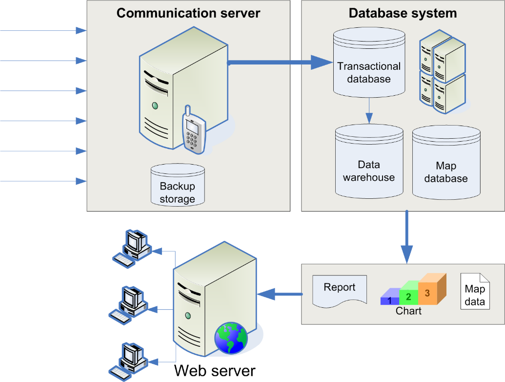
The task of the transactional database is receiving the data from the communication server with high speed and reliability. The data is transferred to a data warehouse which executes several filtering and pre-processing procedures.
The users can access reports, charts and map data on a web-based user interface.
14.4.4. User System
The user system consists of the user computers which are connected to the server system and the user software. It can be stand-alone software with a network database connection or web-application. Nowadays the web-based solutions are dominant (and can be called modern) because of the significant advantages (such as the easier software update and the minimal requirements on the client-side). It is important to note that in the recent years the web-based technologies are developing rapidly, thus made it possible to implement all of the necessary functions and ergonomic graphical interfaces for the effective work. A Fleet Management System can include many user functions [138]:
Vehicle maintenance
Vehicle tracking and diagnostic
Fuel management
Driver management
Tachograph management (Remote download)
Health and safety management
Basically the user system should display the geographical data of the vehicles on a map and the base vehicle data with easy filtering and ordering possibilities.
14.4.4.1. Data displaying, querying, reporting
Large amount of data in itself does not answer the questions of the fleet owner. Suitable business intelligence (BI) solutions are necessary for the data analysis, see [146]. Reporting and displaying system should be designed to support differently the employees with diverse roles considering the executive levels of the company. During the system design phase it is hard to determine all of the necessary and suitable reports. Thus it is important to give the opportunity of the flexible querying for future application.
The system should provide the following output formats:
diagram,
histogram,
statistics,
report.
As a result of the data analysis several outputs can be generated in the above mentioned formats. The generally used outputs are the following:
journey log,
vehicle parameter reports and histograms.
driver style classification,
fuel consumption,
event log,
alarm log,
These outputs can be queried for specific vehicles, drivers (or groups) in specific time periods. In the following figures several examples of the data displaying can be seen.
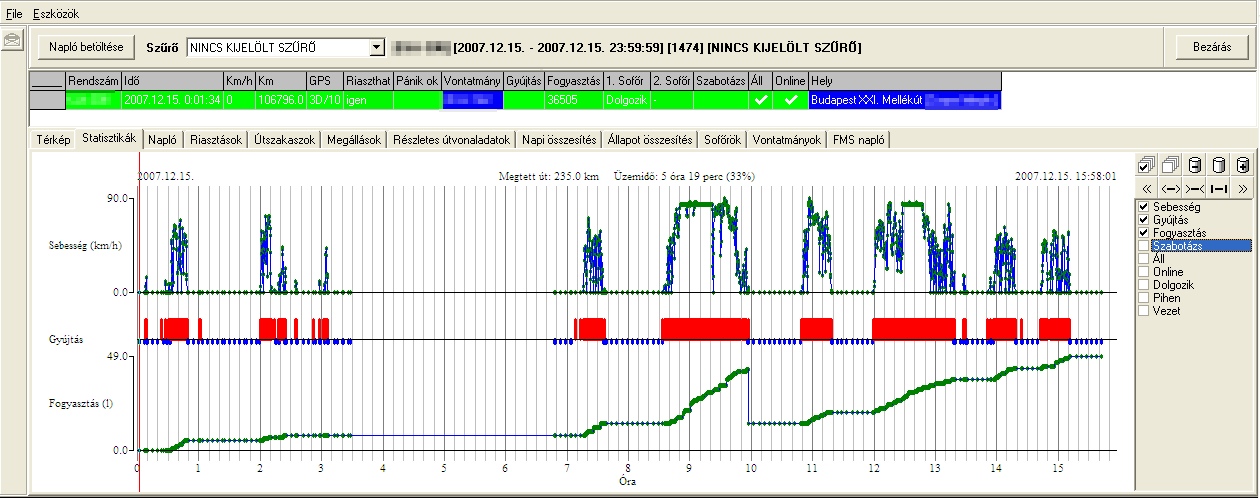
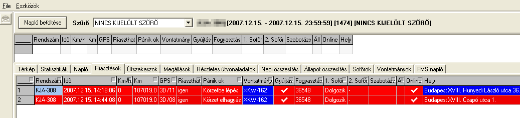
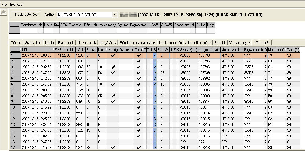
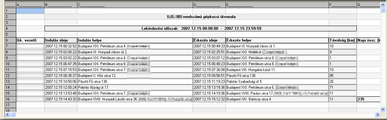
14.4.4.2. Map display
For displaying the vehicles geographical data (actual position and route history) a digital map database and map display engine (collectively referred to as Geographical Information System – GIS) is needed.
The map database stores objects such as roads, lanes, elevation etc. and geocoding information to determine the country, the settlement and the street with the house number.
Basically there are two methods used to store mapping references in a GIS database and to display the map: raster images and vector. The latter technology used geometrical primitives such as points, lines, curves, and shapes or polygons based on mathematical expressions to represent the map objects and support the generation of the map image. Contrary to the raster (or bitmap) image it provides the ability of the clear magnification.
There are several companies offer GIS solutions, technologies and services such as ESRI, Autodesk, ERDAS, MapInfo, Bentley Systems, Intergraph etc.
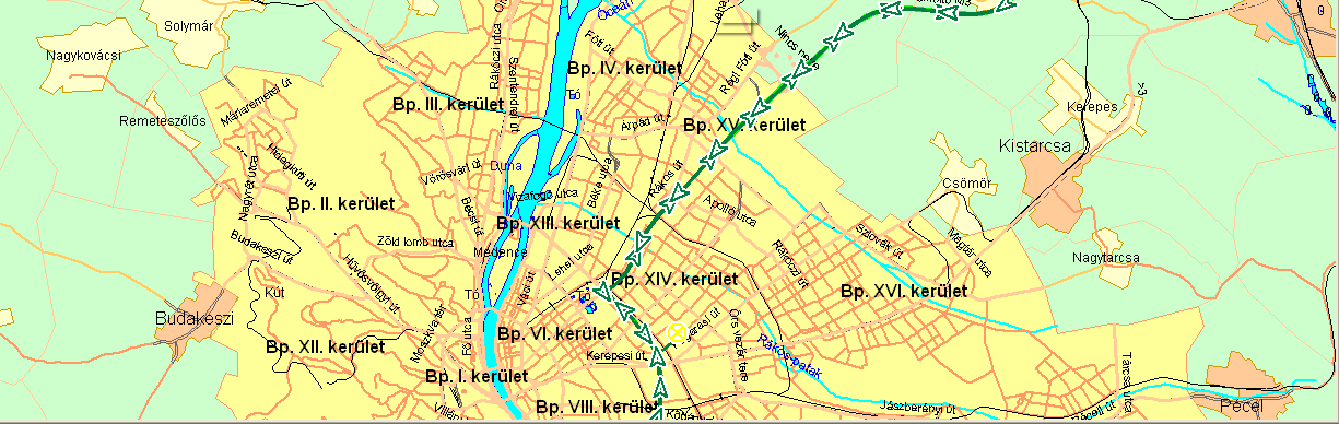
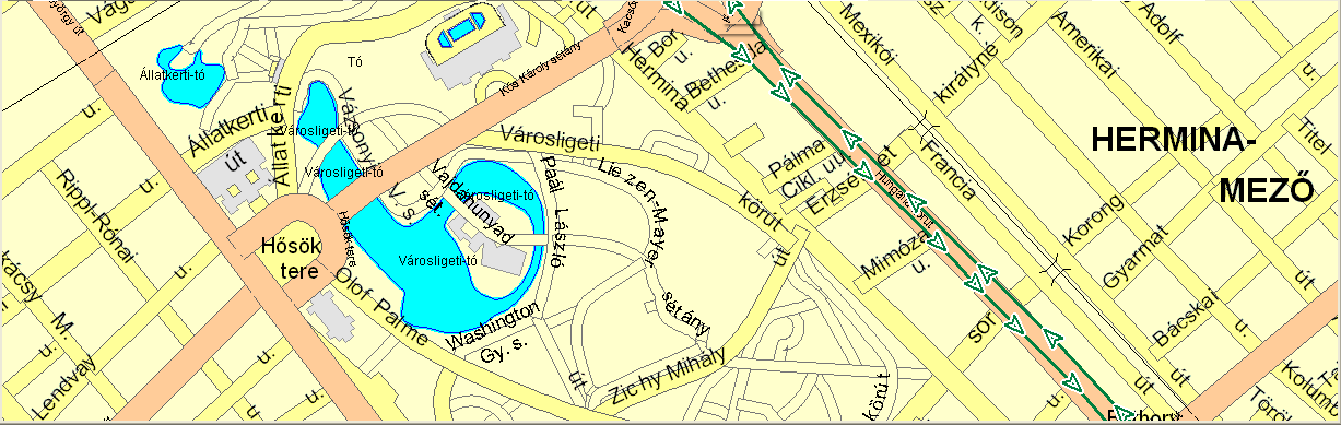
There are several web mapping systems also available for the internet users and more of them provide an API to support the usage in map-based web services. In recent years these services began to gain ground in Fleet Management Systems, because they offers cost-effective licenses, free development platforms and continuously expanding feature list. The most popular services are Google Maps, OpenStreetMap and Bing Maps.
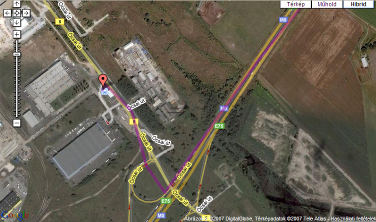
Chapter 15. References
BIBLIOGRAPHY \l 1038
References
[1] Consolidated Resolution On Road Traffic. 2010.
[2] Road fatalities in the EU since 2001, CARE (EU road accident database). 2010.
[3] A Challenging Start towards the EU 2020 Road Safety Target.
[4] Roadmap for moving to a low-carbon economy in 2050.
[5] Euro 6 Emissions Legislation. 2014.
[6] Continental Automotive GmbH and partners. HAVEit- The future of driving, Final Report. 2011.
[7] Driving without a Driver – Volkswagen presents the “Temporary Auto Pilot”. 2011.
[8] Heading for Europe's motorways in a highly automated BMW.
[9] Toyota to Launch Advanced Driving Support System Using Automated Driving Technologies in Mid-2010s. 2013.
[10] IEEE News Releases. 2012.
[11] Google gets first self-driven car license in Nevada. 2012.
[12] What we’re driving at. 2010.
[13] Now Mercedes-Benz Is Promising A Self-Driving Car By 2020. 2013.
[14] Proceedings of the Intelligent Components for Autonomous and Semi-Autonomous Vehicle, pp. 1–5.. Tolouse. Integrated vehicle control systems. 1995.
[15] IEEE Vehicle Power and Propulsion Conference. Harbin, China. Integrated vehicle dynamics control: State-of-the art review. 2008.
[16] Vehicle System Dynamics, vol. 40, pp. 157–190.. Integrated control methodologies for road vehicles. 2003.
[17] Vehicle System Dynamics, vol. 35 pp. 227–289.. Intelligent electronic systems in commercial vehicles for enhanced traffic safety. 2001.
[18] IFAC World Congress. Seoul, Korea. Attitude and handling improvements trough gain-scheduled suspensions and brakes control. 2008.
[19] International Journal of Vehicle Design, vol. 36, pp. 1–12.. Integrated vehicle dynamics control using active brake, steering and suspension systems. 2004.
[20] Mindentudás Egyeteme. Budapest. Intelligens járművek. 2005.
[21] MOSATT 2011: Modern Safety Technologies in Transportation. Kosice, Slovakia. Fault Injection - A Simulation Based Safety Analysis Method for Vehicle Control System Development. 2011.
[22] Springer Verlag: FISITA 2012 World Automotive Congress. Beijing, China. Development of a Vehicle Simulator Based on a Real Car for Research and Education Purposes, F2012-E12-015. 2012.
[23] A jövő járműve – Járműipari innováció, Vol. 5. No 1-2.. Budapest HU ISSN 1788-2699. Korszerű autonóm járműirányítási rendszerek szimulációalapú analízise hibainjektálási módszerrel. 2010.
[24] Közlekedéstudományi Szemle, Vol. 62. No 5. 2012. augusztus, pp. 41-47, ISSN 1788-2699. Budapest. Szimulációs módszertan a magasan automatizált járműfunkciók biztonsági analíziséhez. 2012.
[25] DaimlerChrysler AG and partners. PEIT - Powertrain Equipped with Intelligent Technologies, Final Report. 2005.
[26] IEEE Trans. on Control Systems Technology pp. 1–10.. A robust controller interpolation design technique. 2010.
[27] Joint 48th IEEE Conference on Decision and Control and 28th Chinese Control Conference. Shanghai. Multi-loop interactive control motivated by driver in- the-loop vehicle dynamics controls: The framework. 2009.
[28] “Geometric control theory and linear switched systems,” European Journal of Control, vol. 15, no. 3/4, pp. 378–388.. 2009..
[29] Automotive Radars: Applications and Benefits. 2011.
[30] Hihg Performance Automotive Millimeter Wave Radar System. 1995.
[31] Long-Distance Car Radar. 2011.
[32] Ultrasonic Basics. 2013.
[33] Laurin Publishing Co. Inc.. CCD vs. CMOS. 2001. PHOTONICS SPECTRA.
[34] Elsevier Inc.. Computer and Machine Vision: Theory, ALgorithms, Practicalities. Fourth Edition. 2012.
[35] Bosch Automotive Technology: Stereo Video Camera.
[36] Imaging: The road ahead for car night-vision. 12-13. 2006. Nature Photonics.
[37] Autoliv Visionary.
[38] Autonomous Car Technology.
[39] Ibeo Lux HD Date Sheet. 2013.
[40] Velodyne HDL-64E Datasheet. 2012.
[41] The Global Positioning System. 2014.
[42] Global Navigation Satellite System (GLONASS) Overview. 2010.
[43] The Future - Galileo. 2013.
[44] The System: Vistas from the Summit. 2010.
[45] China Releases Public Service Performance Standard for BeiDou. 2014.
[46] The present - EGNOS. 2013.
[47] High-End DGPS and RTK systems, Periodic Report. 2010.
[48] Assisted GPS, A Low-Infrastructure Approach. 46-51. 2002. GPS World.
[49] IFAC. . DESIGN AND DEVELOPMENT OF AN ADAPTIVE INTEGRATED DRIVER-VEHICLE INTERFACE: OVERVIEW OF THE AIDE PROJECT. 2005.
[50] ITS World Congress. London. . The AIDE adaptive and integrated HMI design: the concept of the Interaction Communication Assistant. 2006.
[51] BMW Insights. 2014.
[52] Brake pedal feel simulator. 2007.
[53] WHITE PAPER - TOUCH SCREENS IN INDUSTRIAL COMPUTER SYSTEMS. 20414.
[54] What Are The Differences Between Capacitive & Resistive Touchscreens?. 2012.
[55] Touchscreens or Human Machine Interface (HMI). 2012.
[56] Dragon Drive: Hands on the wheel, eyes on the road.
[57] Flat Panel Displays. 2014.
[58] OLED-Info. 2004.
[59] GM’s Full Windshield HUD Technology Explained. 2010.
[60] UNECE World Forum for Harmonization of Vehicle Regulations (WP. 29). 2014.
[61] Drowsiness-Detection System. 2014.
[62] University of Iowa. Detecting driver distraction, PhD dissertation. 2009.
[63] Autonomous Driving Technologies for Advanced Driver Assist System, Toyota Motor Corporation. 2013.
[64] 2013.
[65] Ford Active Park Assist. 2010.
[66] IEEE/RSJ International Conference on Intelligent Robots and Systems (IROS 2013). Tokyo. . A Fast Motion Planning Algorithm for Car Parking Based on Static Optimization. 2013.
[67] Driver assistance systems of tomorrow. 2012.
[68] Lane Keeping Assist. 2014.
[69] Active Lane Keeping Assist. 2014.
[70] Toyota Autonomous Driving. 2014.
[71] Semi-Autonomous Nissan Leaf Cleared For Road Test In Japan. 2013.
[72] 4th IEEE Conference on Intelligent Transportation Systems. Oakland. . Road grade and vehicle parameter estimation for longitudinal control using GPS.. 2001.
[73] Intelligent Vehicle Symposium IEEE. . Real time obstacle detection in stereovision on non flat road geometry through "v-disparity" representation. 2002.
[74] Real-time identification of road-bank angle using differential GPS. 589-599. 2004. IEEE Transactions on Control Systems Technology.
[75] Road slope and vehicle mass estimation using Kalman filtering. 12-23. 2002. Vehicle System Dynamics Supplement.
[76] Midwest Research Institute. Kansas City. Prediction of the expected safety performance of rural two-lane highways, Technical Report. 1971.
[77] Texas Transportation Institute. Texas. The relationship of vehicle paths to highway curve design, Research Study. 1971.
[78] Validation of the circular trajectory assumption in critical speed, SAE Technical Paper. 2005.
[79] Society of Automotive Engineers (SAE). An analytical assessment of the critical speed formula, Research Report. 1997..
[80] TRL Limited. New and improved accident reconstruction techniques for modern vehicles equipped with esc systems, Project Report. 2007.
[81] Slip-based tire-road friction estimation. 6. 1087-1099. 1997. Automatica.
[82] On-board road condition monitoring system using slip-based tyre-road friction estimation and wheel speed signal analysis. 1. 129-146. 2007. Automatica.
[83] Dynamic friction model-based tire-road friction estimation and emergency braking control. 1. 22-32. 2005. Journal of Dynamic Systems, Measurement and Control.
[84] 6th International Conference on Managing Pavements. . A method to evaluate side friction in horizontal curves, using supply-demand concepts. 2004.
[85] Practical vehicle rollover avoidance control using energy method. 4. 323-337. 2008. Vehicle System Dynamics.
[86] Modeling of rollover sequences. 209-216. 2003. Control Engineering Practice.
[87] Slow active suspension control for rollover prevention. 29-36. 2013. Journal of Terramechanics.
[88] SAE. Warrendale. Fundamentals of Vehicle Dynamics. 1994.
[89] Sensitivity of Contact Electronic Throttle Control Sensor to Control System Variation, SAE Technical Paper Series. 2006.
[90] Maróti Könyvkiadó. Budapest. Gépjárművek buszhálózatai (CAN, VAN, LIN, Byteflight, FlexRay, MOST, Bluetooth és egyéb rendszerek). 2013.
[91] Bosch CAN Specification Version 2.0. 1991.
[92] International Standard 11898-2, Road vehicles Controller area network (CAN) - High-speed medium access unit. 2003.
[93] http://www.autosec.org/pubs/cars-usenixsec2011.pdf. Comprehensive Experimental Analyses of Automotive Attack Surfaces.
[94] http://www.autosec.org/pubs/cars-oakland2010.pdf. Experimental Security Analysis of a Modern Automobile. 2011.
[95] https://hacktivity.com/hu/letoltesek/archivum/303/. Adventures in Automotive Networks and Control Units. 2012.
[96] Steer By Wire. 2013.
[97] ELECTRICALLY POWERED STEERING. 2014.
[98] Active Steering. 2013.
[99] Nissan Pioneers First-Ever Independent Control Steering Technology. 2012.
[100] Budapest University of Technology and Economics. Budapest. Tire-, Braking- and Driving Mechanics, Mechatronic Safety Systems. 2012.
[101] Mindentudás Egyeteme. Budapest. Intelligens járművek. 2005..
[102] Mercedes cancels by-wire brake system; decision a blow to technology's future. 2005.
[103] Brakes of the Future Will Slow Down the Vehicle Electrically. 2001.
[104] http://www.citroen.com.au/about-citroen/technology/comfort/sensodrive-gearbox. Sensodrive Gearbox. 2014.
[105] http://www.zf.com/media/media/document/corporate_2/downloads_1/flyer_and_brochures/powertrain_and_suspension_components/03_ZF_Sachs_Product_Information_PC_A_Automated_Manual_Transmission_en_ebook.pdf. Automated Manual Transmission .
[106] http://auto.howstuffworks.com/dual-clutch-transmission.htm. How Dual-clutch Transmissions Work. 2014.
[107] Voith. http://resource.voith.com/vt/publications/downloads/483_e_483_e_g_1747_e_diwa5_2012-08_screen.pdf. Combining Ride Comfort with Economy. 2014.
[108] http://www.nissan-global.com/EN/TECHNOLOGY/OVERVIEW/cvt.html. CVT Transmission. 2014.
[109] LVMM - The Localized Vehicular Multicast Middleware: a Framework for Ad Hoc Inter-Vehicles Multicast Communications. 2005.
[110] IETF. Mobile Ad hoc Networking (MANET): Routing Protocol Performance Issues and Evaluation Considerations. 1999.
[111] Securing vehicular ad hoc networks. 39-68. 2007. Journal of Computer Security.
[112] IEEE Vehicular Technology Conference. Singapore. . IEEE 802.11p: Towards an International Standard for Wireless Access in Vehicular Environments. 2008.
[113] ITS Car-toCar Communications Standards, NIST-CDV Workshop on ITS. 2010.
[114] Cars that talk: Commission earmarks single radio frequency for road safety and traffic management. 2008.
[115] DSRC Implementation Guide: A guide to users of SAE J2735 message sets over DSRC . 2010.
[116] CAR 2 CAR Communication Consortium Manifesto. 2007.
[117] http://www.its.dot.gov/research/v2i.htm#one. 2011.
[118] Adaptive Frequency Hopping for Reduced Interference between Bluetooth® and Wireless LAN. 2003.
[119] What is Bluetooth technology.
[120] Mobile technologies GSM. 2014.
[121] UMTS. 2014.
[122] European Commission Joint Research Centre Institute for Prospective Technological Studies. Road Traffic Data: Collection Methods and Applications. 2008.
[123] Int. Conf. on Traffic and Transport Psychology. Washington DC. . Electronically coupled truck convoys and driver's response from the project konvoi. 2008.
[124] 17th World Congress on Intelligent Transport Systems. Busan. . Operating platoons on public motorways: An introduction to the sartre platooning programme. 2010.
[125] Int. Conf. on on Advanced Driver Assistance Systems. Birmingham. . Promote-chauffeur ii and 5.8 ghz vehicle to vehicle communications system. 2001.
[126] Innovation of distributed driver assistance systems for commercial vehicle platform. 2011.
[127] String stability of interconnected systems: An application to platooning in automated highway systems, PhD dissertation. 1994.
[128] Road surface description and vehicle response. 25-35. 1979. Int. J. of Vehicle Design.
[129] Power spectral density of road profiles. 409-415. 2001. Vehicle System Dynamics.
[130] Adaptive control of vehicle suspension. 57-74. 1987. Vehicle System Dynamics.
[131] Multiobjective optimal suspension control to achieve integrated ride and handling performance. 807-821. 2002. IEEE Transactions on Control Systems Technology.
[132] Plug and play control: Control technology towards new challenges. 3. 2009. European Journal of Control.
[133] Integrated control methodologies for road vehicles. 157-190. 2003. Vehicle System Dynamics.
[134] Integrated vehicle control using steering and brakes. 534-541. 2006. International Journal of Control.
[135] Integrated control of active suspension system and electronic stability programme using hierarchical control strategy: theory and experiment. 381-397. 2011. Vehicle System Dynamics.
[136] Conference on Decision and Control. Cancun. . Design of reconfigurable and fault-tolerant suspension systems based on LPV methods. 2008.
[137] FISITA. Budapest. . Complex Fleet Management Requirements for Fuel Transportation. 2010.
[138] Fleet Management System. 2013.
[139] IFFK. Budapest. . Jármű CAN adatok flottamenedzsment célú felhasználási lehetőségei MAN és MB haszongépjárművek esetén. 2009.
[140] CAN bus communication. 2013.
[141] FMS Standard. 2013.
[142] FMS Gateway.
[143] ISO/IEC 7498-1. 1994.
[144] User Datagram Protocol (UDP). 1980.
[145] Transmission Control Protocol. 1981.
[146] IFFK. Budapest. . Üzleti intelligencia rendszerek fejlesztése a hatékony flottamenedzsment szolgálatában. 2011.
[147] Pepperl+Fuchs: Ultrasonic Sensors. 2005.